AHL 4.15 — Linear combinations of normal variables(正規分布にしたがう確率変数の一次結合)
- 独立な normal の和や差が、やはり normal になると言える。
- その平均と variance(分散)を出して、\(N(\mu,\ \sigma^{2})\) の形に書ける。
- そこから normCdf で確率を求められる。
- \(\bar{X} \sim N\!\left(\mu,\ \dfrac{\sigma^{2}}{n}\right)\) を使い、sample(標本)平均の確率を求められる。
- central limit theorem(中心極限定理)が何を言っているかを説明できる。
- もとの分布が normal と分からないとき、標本数が十分に大きければ \(\bar{X}\) を近似的に normal として扱えると分かる。
The idea
1. Linear combinations of normal variables(正規分布にしたがう確率変数の一次結合)
AHL 4.14 では、独立な確率変数を足すと、平均も分散も足し算できることを学びました。ただし、平均と分散だけでは、分布の形は分かりません。 ここでは、normal distribution(正規分布)にしたがう確率変数の和や差について、確率を求める方法を学びます。
linear combination(一次結合)とは
\(X + Y\)、\(2X - Y\)、\(\dfrac{X_1 + \cdots + X_n}{n}\) のように、確率変数に定数をかけて足し合わせたものを linear combination(一次結合)といいます。
「和」「差」「標本平均」は、すべて一次結合の例です。 ですからこのページの \(3\) つの話題は、どれも \(1\) つの考え方で扱えます。
\(X_1,\ \ldots,\ X_n\) が互いに独立で、
\[ X_i \sim N(\mu_i,\ \sigma_i^{2}) \]
にしたがうとします。このとき、定数 \(a_1,\ \ldots,\ a_n\) をかけて足し合わせて作った新しい確率変数
\[ Y = a_1X_1 + \cdots + a_nX_n \tag{1}\]
も normal distribution にしたがい、
\[ E(Y) = a_1\mu_1 + \cdots + a_n\mu_n \tag{2}\]
\[ \text{Var}(Y) = a_1^{2}\sigma_1^{2} + \cdots + a_n^{2}\sigma_n^{2} \tag{3}\]
となります。
平均では係数をそのまま使いますが、分散では係数を \(2\) 乗します。 差のときも分散が足し算になるのは、この \(2\) 乗によって負の符号が消えるためです。
「normal を入れれば、normal が出てくる」——これだけです。どんな分布でもこうなるわけではありません(独立な \(2\) つの Poisson の和が Poisson になるのは、AHL 4.17 の別の規則です)。
2. Sum of independent normal variables(独立な正規分布の和)
まず、和の分布を求めます。独立な確率変数を足すときは、standard deviation(標準偏差)を直接足すのではなく、まず分散を足します。 最後に平方根を取って標準偏差へ戻します。
主菜の質量 \(M \sim N(250,\ 8^{2})\) と副菜の質量 \(S \sim N(180,\ 6^{2})\) が独立なとき、合計 \(M + S\) の分布を求めてみます。
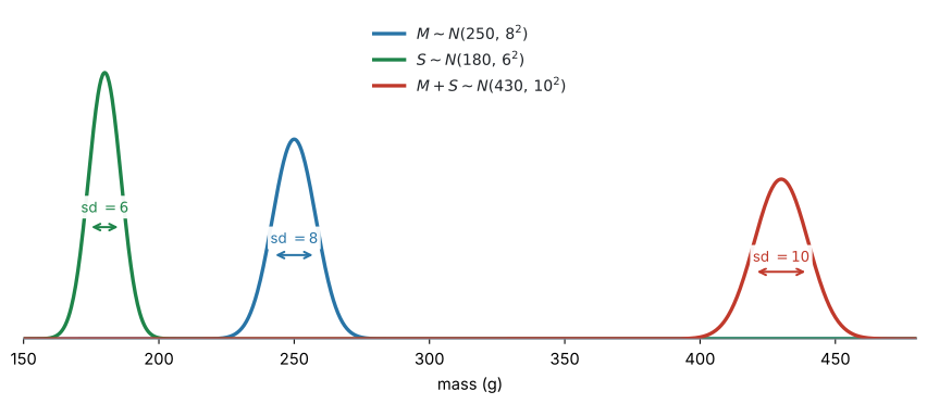
平均は、そのまま足します。
\[ E(M + S) = 250 + 180 = 430 \]
独立なので、分散も足します。標準偏差ではありません。
\[ \text{Var}(M + S) = 8^{2} + 6^{2} = 100 \]
標準偏差は、分散の正の平方根です。
\[ \sigma_{M+S} = \sqrt{100} = 10 \]
したがって
\[ M + S \sim N(430,\ 100) \]
です。図 1 のとおり、\(M\) と \(S\) を足して出てくるのも normal distribution です。
\(N(\mu,\ \sigma^{2})\) のカッコの \(2\) 番目は、分散です。 \(N(430,\ 100)\) の \(100\) は分散で、標準偏差の \(10\) を書くのではありません。
3. Three-step method(\(3\) つの手順)
この項目の問題は、ほとんど同じ形をしています。次の \(3\) つの手順で解けます。
\(M + S\) の例なら、\(E = 430\) → \(\text{Var} = 100\) → \(M + S \sim N(430,\ 100)\) と書いて、\(\sigma = 10\) を normCdf へ、という流れです。
\(1\) と \(2\) は AHL 4.14、\(3\) の後半は SL 4.9 です。 このページが新しく足しているのは、手順 \(3\) の前半、「normal だと言ってよい」という一歩だけです。
normCdf に入れるのは、標準偏差です
GDC の normCdf に入力するのは mean(平均)と standard deviation(標準偏差)です。分散を求めた後、平方根を取るのを忘れないでください。
電卓に入れる前に、求めた分布を \(1\) 行書く習慣をつけてください。
\(M + S \sim N(430,\ 100)\)
ここに点が付き、\(\sigma\) と \(\sigma^{2}\) の取りちがえも防げます。
例題 1 In a school canteen, the mass of a main dish, in grams, is \(M \sim N(250,\ 8^{2})\) and the mass of a side dish is \(S \sim N(180,\ 6^{2})\). The two masses are independent.
A meal consists of one main dish and one side dish. Let \(T = M + S\) be the total mass of a meal.
(a) State the distribution of \(T\), giving its mean and variance.
(b) Find \(P(T > 445)\).
(c) Find the probability that the total mass of a meal is between \(420\) g and \(445\) g.
日本語訳
ある学校の食堂で、主菜の質量(グラム)は \(M \sim N(250,\ 8^{2})\)、副菜の質量は \(S \sim N(180,\ 6^{2})\) です。この \(2\) つの質量は独立です。
\(1\) 食は、主菜 \(1\) つと副菜 \(1\) つからなります。\(1\) 食の合計質量を \(T = M + S\) とします。
(a) \(T\) の分布を、平均と分散を示して述べなさい。
(b) \(P(T > 445)\) を求めなさい。
(c) \(1\) 食の合計質量が \(420\) g から \(445\) g のあいだになる確率を求めなさい。
(a) 第3節の \(3\) ステップのうち、\(1\) と \(2\) です。\(1\) 食の合計質量を \(T = M + S\) とおきます。
平均は、係数をそのまま使います。
\[ E(T) = 250 + 180 = 430 \]
分散は、係数を \(2\) 乗して足します。ここでは係数がどちらも \(1\) なので、\(8^{2}\) と \(6^{2}\) をそのまま足します。standard deviation ではなく、variance を足すところが要点です。
\[ \text{Var}(T) = 8^{2} + 6^{2} = 64 + 36 = 100 \]
\(M\) も \(S\) も normal で、独立なので、\(T\) は exactly normal です(第1節)。
\[ T \sim N(430,\ 100) \]
検算。 \(\sigma = \sqrt{100} = 10\) です。\(8 + 6 = 14\) ではありません(第2節)。
(b) \(\sigma = 10\) を normCdf に入れます。\(100\) ではありません。
\(\texttt{normCdf}\left(445,\ \infty,\ 430,\ 10\right)\)
\[ P(T > 445) = 0.0668 \]
\(1\) 食の合計質量が \(445\) g を超えるのは、およそ \(100\) 食のうち \(7\) 食です。
(c) 両端があるので、normCdf の \(2\) か所を埋めるだけです。
\(\texttt{normCdf}\left(420,\ 445,\ 430,\ 10\right)\)
\[ P(420 < T < 445) = 0.775 \]
\(1\) 食のおよそ \(77\%\) が、\(420\) g から \(445\) g のあいだに入ります。
(a) \[ E(T) = 250 + 180 = 430 \] \[ \text{Var}(T) = 8^{2} + 6^{2} = 100 \] \[ T \sim N(430,\ 100) \]
(b) \[ P(T > 445) = 0.0668 \]
(c) \[ P(420 < T < 445) = 0.775 \]
ここからは、この問題の解答ではなく、同じ考え方を別の場面に使う話です。同じ分布のものを \(2\) つ足すこともできます。
\(X \sim N(250,\ 8^{2})\) のコーヒーを \(2\) 杯なら
\[ X_1 + X_2 \sim N(500,\ 128), \qquad \sigma = \sqrt{128} = 11.3 \]
で、\(P(X_1 + X_2 > 510) = 0.188\) です。
ここで \(2X\) としてはいけません。 \(2X\) なら分散は \(4 \times 64 = 256\)、\(\sigma = 16\) になり、\(P(2X > 510) = 0.266\) と別の答えになります(AHL 4.14)。
\(2\) 杯あるのか、\(1\) 杯を \(2\) 倍するのか。問題文で数えてください。
4. Difference of two normal variables(\(2\) つの正規分布の差)
次は、差の分布です。差も一次結合の \(1\) つで、平均は引いて、分散は足します。
\(X\) と \(Y\) が独立のとき、差を表す新しい確率変数 \(D = X - Y\) は、\(Y\) の係数を \(-1\) とする一次結合
\[ D = X + (-1)Y \]
と書けます。平均は係数をそのまま使うので
\[ E(D) = E(X) - E(Y) \]
です。分散では係数を \(2\) 乗するので、\((-1)^{2} = 1\) となり
\[ \text{Var}(D) = \text{Var}(X) + (-1)^{2}\text{Var}(Y) = \text{Var}(X) + \text{Var}(Y) \tag{4}\]
です。差でも、分散は足し算です。 この式は、\(X\) と \(Y\) が独立である場合に使えます(AHL 4.14)。
たとえば \(X \sim N(20,\ 3^{2})\) と \(Y \sim N(16,\ 4^{2})\) が独立なら、\(E(D) = 20 - 16 = 4\)、\(\text{Var}(D) = 9 + 16 = 25\) で、\(D \sim N(4,\ 25)\) です。
「\(A\) のほうが大きい確率」は、差で考えます
「\(A\) が \(B\) より大きい確率を求めなさい」(Find the probability that A is greater than B)と聞かれたら、\(D = A - B\) という新しい確率変数を作ります。次の言いかえができるからです。
\[ A > B \iff A - B > 0 \iff D > 0 \]
\(A\) のほうが大きいことと、\(D\) が正であることは、同じ出来事です。ですから
\[ P(A > B) = P(A - B > 0) = P(D > 0) \tag{5}\]
と書きかえられます。\(A\) と \(B\) が独立な normal なら、\(D\) も normal です(第1節)。\(2\) つの分布を見くらべるのではなく、\(D\) についての \(1\) つの normal distribution の問題に変える——これがこの型の考え方です。
例題 2 The lifetime of a battery of brand A, in hours, is \(X \sim N(30,\ 4^{2})\). The lifetime of a battery of brand B is \(Y \sim N(27,\ 3^{2})\). All lifetimes are independent.
One battery of each brand is chosen at random. Let \(D = X - Y\).
(a) State the distribution of \(D\).
(b) Find the probability that the brand A battery lasts longer than the brand B battery.
(c) Find the probability that the brand A battery lasts at least \(5\) hours longer than the brand B battery.
(d) Explain why the standard deviation of \(D\) is not \(4 - 3 = 1\).
日本語訳
ブランド A の電池の寿命(時間)は \(X \sim N(30,\ 4^{2})\)、ブランド B の電池の寿命は \(Y \sim N(27,\ 3^{2})\) です。すべての寿命は独立です。
lifetime は「寿命」、at least は「少なくとも」という意味です。
各ブランドから電池を \(1\) 個ずつ無作為に選びます。\(D = X - Y\) とします。
(a) \(D\) の分布を述べなさい。
(b) ブランド A の電池のほうが、ブランド B の電池より長持ちする確率を求めなさい。
(c) ブランド A の電池が、ブランド B の電池より少なくとも \(5\) 時間長持ちする確率を求めなさい。
(d) \(D\) の標準偏差が \(4 - 3 = 1\) にならない理由を説明しなさい。
(a) \(D = X - Y = X + (-1)Y\) とおきます。平均は係数をそのまま使い、分散は係数を \(2\) 乗します(式 4)。
\[ E(D) = 30 - 27 = 3 \]
\[ \text{Var}(D) = 4^{2} + (-1)^{2} \times 3^{2} = 16 + 9 = 25 \]
\(X\) も \(Y\) も normal で、独立なので、\(D\) は exactly normal です。
\[ D \sim N(3,\ 25) \]
\(N(3,\ 25)\) の \(25\) は分散なので、標準偏差は \(\sigma = \sqrt{25} = 5\) です。normCdf には \(5\) を入れます。
(b) 「A のほうが長い」は「\(D\) が正」ということです(式 5)。
\[ P(X > Y) = P(D > 0) \]
\(\texttt{normCdf}\left(0,\ \infty,\ 3,\ 5\right)\)
\[ P(D > 0) = 0.726 \]
ブランド A のほうが長持ちするのは、およそ \(73\%\) です。
検算。 \(E(D) = 3 > 0\) なので、確率は \(0.5\) より大きくなるはずです ✓
(c) at least 5 hours longer は \(D \geq 5\) です。
\(\texttt{normCdf}\left(5,\ \infty,\ 3,\ 5\right)\)
\[ P(D \geq 5) = 0.345 \]
\(5\) 時間以上長持ちするのは、およそ \(34\%\) です。
(d) 足すのは標準偏差ではなく分散で、しかも差のときも足します。\(Y\) の係数 \(-1\) が \(2\) 乗されて \(+1\) になるからです。\(Y\) を引いても \(Y\) のばらつきは消えず、\(Y\) がぶれれば \(X - Y\) もぶれるので、\(2\) つのばらつきは打ち消し合わずに重なります。
試験ではこう書く
Variances add, not standard deviations, and they add for a difference as well: \(\text{Var}(D) = 4^{2} + (-1)^{2} \times 3^{2} = 25\), so the standard deviation is \(\sqrt{25} = 5\).
Subtracting \(Y\) does not remove the variability of \(Y\).
(a) \[ E(D) = 30 - 27 = 3, \qquad \text{Var}(D) = 4^{2} + (-1)^{2} \times 3^{2} = 25 \] \[ D \sim N(3,\ 25) \]
(b) \[ P(X > Y) = P(D > 0) = 0.726 \]
(c) \[ P(D \geq 5) = 0.345 \]
(d) Variances add rather than standard deviations, and they add for a difference as well as for a sum: \(\text{Var}(D) = 4^{2} + (-1)^{2} \times 3^{2} = 25\), so \(\sigma = 5\). Subtracting \(Y\) does not remove the variability of \(Y\).
5. Distribution of the sample mean \(\bar{X}\)(標本平均 \(\bar{X}\) の分布)
この項目のもう \(1\) つの中心が、sample mean(標本平均)\(\bar{X}\) の分布です。\(\bar{X}\) は「エックス・バー」と読みます。\(\bar{X}\) も一次結合なので、第1節の性質がそのまま使えます。
population(母集団)が \(N(\mu,\ \sigma^{2})\) のとき、そこから独立に \(n\) 個を取り出します。\(1\) 回目、\(2\) 回目、……で得られる値を表す確率変数を \(X_1,\ X_2,\ \ldots,\ X_n\) とすると、どれも \(X_i \sim N(\mu,\ \sigma^{2})\) です。たとえば身長なら、\(X_1\) は「\(1\) 人目に選ばれる人の身長」で、実際に測って出た \(168\) cm はその observed value(観測値)です。
この \(n\) 個の平均を表す新しい確率変数が、sample mean \(\bar{X}\) です。
\[ \bar{X} = \frac{X_1 + \cdots + X_n}{n} = \frac{1}{n}X_1 + \cdots + \frac{1}{n}X_n \]
つまり \(\bar{X}\) は、各 \(X_i\) の係数が \(\dfrac{1}{n}\) である linear combination(一次結合)です。
平均は、係数をそのまま使います。
\[ \begin{aligned} E(\bar{X}) &= \frac{1}{n}\mu + \cdots + \frac{1}{n}\mu \\ &= n\left(\frac{1}{n}\right)\mu \\ &= \mu \end{aligned} \]
\(\bar{X}\) の平均は、population mean(母平均)\(\mu\) と同じです。
分散では、係数 \(\dfrac{1}{n}\) を \(2\) 乗します。各 \(X_i\) は独立で、分散はどれも \(\sigma^{2}\) なので
\[ \begin{aligned} \text{Var}(\bar{X}) &= \left(\frac{1}{n}\right)^{2}\text{Var}(X_1) + \cdots + \left(\frac{1}{n}\right)^{2}\text{Var}(X_n) \\ &= n\left(\frac{1}{n}\right)^{2}\sigma^{2} \\ &= n \cdot \frac{1}{n^{2}}\sigma^{2} \\ &= \frac{\sigma^{2}}{n} \end{aligned} \]
となります。\(\dfrac{1}{n}\) 倍ではありません。
\[ \boxed{\ \text{Var}(\bar{X}) = \frac{\sigma^{2}}{n}\ } \]
標準偏差は、その平方根です。
\[ \sigma_{\bar{X}} = \sqrt{\frac{\sigma^{2}}{n}} = \frac{\sigma}{\sqrt{n}} \tag{6}\]
また、独立な normal の一次結合も normal なので
\[ \boxed{\ \bar{X} \sim N\!\left(\mu,\ \frac{\sigma^{2}}{n}\right)\ } \tag{7}\]
です。この \(\dfrac{\sigma}{\sqrt{n}}\) を standard error(標準誤差)といいます。\(n\) が大きいほど standard error は小さくなり、\(\bar{X}\) は \(\mu\) の近くに集まりやすくなります。
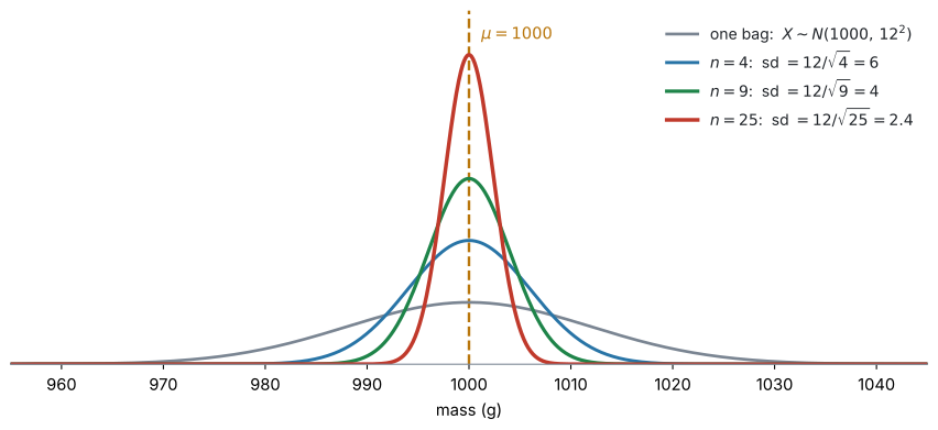
中心は動かず、幅だけが狭くなります
図 2 の \(4\) つの曲線は、すべて \(\mu = 1000\) を中心にしています。違うのは幅だけです。標本の数が増えると、偶然によるばらつきが平均の中で打ち消し合うため、\(\bar{X}\) は母平均 \(\mu\) の近くに集まりやすくなります(AHL 4.14)。
\(\sigma / n\) ではありません。 分散が \(\sigma^{2}/n\) なので、平方根をとると分母は \(\sqrt{n}\) になります。\(\sigma = 12\)、\(n = 9\) なら \(\sigma_{\bar{X}} = \dfrac{12}{3} = 4\) で、\(\dfrac{12}{9}\) ではありません。
\(1\) 袋の質量は \(1000\) g から \(20\) g ずれることもあります。しかし \(9\) 袋の平均が \(20\) g もずれることは、めったにありません。重い袋と軽い袋が打ち消し合うからです。これが、標本をたくさんとる理由です。
問題文が
the mass of one bag… \(X \sim N(1000,\ 12^{2})\)、\(\sigma = 12\)the mean mass of nine bags… \(\bar{X} \sim N(1000,\ 16)\)、\(\sigma = 4\)the total mass of nine bags… \(\sum X \sim N(9000,\ 1296)\)、\(\sigma = 36\)
の \(3\) つを区別します。\(\sigma\) は \(12\)、\(4\)、\(36\) と全部違います。 平均のほうは one と mean がどちらも \(1000\) で、total だけ \(9000\) です。
平均が同じでも \(\sigma\) が違う——one と mean の取りちがえが危ないのは、ここです。one なのか mean なのか total なのか、丸で囲んでから計算を始めてください。
例題 3 The mass of a bag of sugar, in grams, is normally distributed with mean \(1000\) and standard deviation \(12\).
(a) Find the probability that a randomly chosen bag has a mass less than \(995\) g.
(b) Nine bags are chosen at random. Find the probability that their mean mass is less than \(995\) g.
(c) Comment on the difference between your answers to parts (a) and (b).
日本語訳
砂糖 \(1\) 袋の質量(グラム)は、平均 \(1000\)、標準偏差 \(12\) の正規分布にしたがいます。
(a) 無作為に選んだ \(1\) 袋の質量が \(995\) g 未満である確率を求めなさい。
(b) \(9\) 袋を無作為に選びます。その平均質量が \(995\) g 未満である確率を求めなさい。
(c) (a) と (b) の答えの違いについて述べなさい。
\(1\) 袋の質量を \(X\)、\(9\) 袋の標本平均を \(\bar{X}\) とします。この \(2\) つを、記号でも区別してください。
(a) \(1\) 袋を選ぶ場合なので、\(X \sim N(1000,\ 12^{2}) = N(1000,\ 144)\) をそのまま使います。標準偏差は \(\sigma = 12\) です。
\(\texttt{normCdf}\left(-\infty,\ 995,\ 1000,\ 12\right)\)
\[ P(X < 995) = 0.338 \]
(b) \(9\) 袋の平均を調べる場合なので \(\bar{X}\) です。\(9\) 袋は独立で、もとの \(X\) が normal なので、\(n = 9\) でも \(\bar{X}\) は exactly normal です(式 7)。
\[ \bar{X} \sim N\!\left(1000,\ \frac{144}{9}\right) = N(1000,\ 16) \]
\[ \sigma_{\bar{X}} = \frac{12}{\sqrt{9}} = \frac{12}{3} = 4 \]
\(\texttt{normCdf}\left(-\infty,\ 995,\ 1000,\ 4\right)\)
\[ P(\bar{X} < 995) = 0.106 \]
検算。 \(\sigma\) が \(12\) から \(4\) に小さくなったので、確率も小さくなるはずです ✓
(c) \(9\) 袋の平均のほうが、はるかに起こりにくくなっています。
試験ではこう書く
The probability drops from \(0.338\) to \(0.106\).
For a single bag, one light bag is enough to fall below \(995\) g.
For the mean of nine bags, a light bag tends to be offset by a heavier one, so the mean falls below \(995\) g only if the nine bags are light on average, which is much less likely.
The standard deviation of the mean is \(12/\sqrt{9} = 4\), only a third of the standard deviation of a single bag.
(確率は \(0.338\) から \(0.106\) に下がる。\(1\) 袋なら軽い袋 \(1\) つで \(995\) g を下回るが、\(9\) 袋の平均では軽い袋が重い袋で打ち消されるので、\(9\) 袋そろって軽いときにしか下回らず、はるかに起こりにくい、という意味です。)
(a) \[ X \sim N(1000,\ 144), \qquad P(X < 995) = 0.338 \]
(b) \[ \bar{X} \sim N\!\left(1000,\ \frac{144}{9}\right) = N(1000,\ 16), \qquad \sigma_{\bar{X}} = 4 \] \[ P(\bar{X} < 995) = 0.106 \]
(c) The probability is much smaller for the mean of nine bags (\(0.106\) against \(0.338\)), because the standard deviation of \(\bar{X}\) is \(12/\sqrt{9} = 4\), only one third of that of a single bag. Light bags tend to be offset by heavy ones, so the mean of nine bags stays close to \(1000\) g.
6. Central limit theorem(中心極限定理)
ここまでは、population(母集団)が normal distribution にしたがう場合を考えてきました。しかし、実際のデータの分布は、いつも normal になるとはかぎりません。たとえば待ち時間の分布は、短い値が多く、右側に長く伸びた形になることがあります。
では、もとの分布が normal でない場合、sample mean \(\bar{X}\) はどのような分布になるのでしょうか。
\(1\) 回の測定値と sample mean は、別のものです
同じ population から独立に取り出した \(n\) 個の値を \(X_1,\ X_2,\ \ldots,\ X_n\) とし、その sample mean を
\[ \bar{X} = \frac{X_1 + \cdots + X_n}{n} \]
とします。もとの population が normal でなければ、\(1\) 回の測定値 \(X_i\) の分布も normal ではありません。しかし、\(n\) 個から作った \(\bar{X}\) の分布は、\(n\) が大きくなるにつれて normal distribution に近づいていきます。
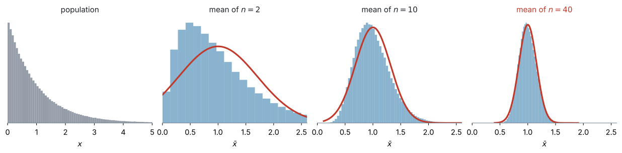
図 3 のいちばん左は、normal ではない population です。右に大きく尾を引いています。その右の \(3\) つは、そこから \(n\) 個を取り出して平均する、ということをくり返して描いた \(\bar{X}\) の分布です。赤い曲線は、それぞれの \(\bar{X}\) と同じ平均・標準偏差をもつ normal distribution です。
- \(n = 2\) … まだ歪んでいます
- \(n = 10\) … normal に近づいてきました
- \(n = 40\) … 赤い normal の曲線にほぼ重なっています
これが central limit theorem(中心極限定理、CLT)です。
同じ population から独立に取り出した標本の sample mean \(\bar{X}\) は、sample size \(n\) が十分に大きいとき、もとの population が normal でなくても、approximately normal distribution(近似的な正規分布)にしたがいます。
population の平均を \(\mu\)、分散を \(\sigma^{2}\) とすると
\[ \boxed{\ \bar{X} \approx N\!\left(\mu,\ \frac{\sigma^{2}}{n}\right)\ } \tag{8}\]
です。平均は \(\mu\)、分散は \(\dfrac{\sigma^{2}}{n}\)、標準偏差は \(\dfrac{\sigma}{\sqrt{n}}\)(standard error)で、第5節とまったく同じです。
平均と分散は、もとが normal でなくてもそのままです(AHL 4.14 から出るので、分布の形は関係ありません)。CLT が足してくれるのは、形が normal に近いという一点だけです。
\(n\) が大きくなると、何が起こるのか
\(n\) が大きくなると \(\dfrac{\sigma}{\sqrt{n}}\) は小さくなり、\(\bar{X}\) は population mean \(\mu\) の近くに集まりやすくなります。同時に、\(\bar{X}\) の分布の形が normal distribution に近づきます。
CLT は「データが normal になる」とは言っていません
CLT は、もとのデータ \(X_i\) の分布が normal になるという定理ではありません。 normal に近づくのは、何度も標本を取って作った sample mean \(\bar{X}\) の分布です。図 3 のいちばん左の形は、\(n\) をどれだけ大きくしても変わりません。変わるのは、その右の \(3\) つのほうです。
どのくらいの \(n\) が必要ですか
試験では、通常 \(n > 30\) を「十分に大きい」とする目安が使われます。ただし、これは数学的な境界ではありません。 分布の偏りが強い場合や outlier(外れ値)が多い場合は、より大きな \(n\) が必要になることがあります。
CLT を使うときは、normal distribution で近似している理由を \(1\) 行書きます。
試験ではこう書く
Since \(n = 40 > 30\), by the central limit theorem, \(\bar{X}\) is approximately normal.
(\(n = 40 > 30\) なので、中心極限定理により \(\bar{X}\) は近似的に正規分布にしたがう、という意味です。)
ここでは、approximately(近似的に)と書くことが大事です。もとの population が normal だと分かっている場合を除き、exactly normal とは言えません。
7. Sample mean and sample total(平均で解くか、合計で解くか)
平均についての問題は、合計の問題に言いかえても同じ答えになります。例で確かめます。
\(40\) 人の待ち時間を調べます。\(i\) 人目の待ち時間を \(X_i\) とし、\(1\) 人あたり \(\mu = 4.2\)、\(\sigma = 2.5\) とします。\(1\) 人分の待ち時間が normal distribution にしたがうとは分かっていません。求めるのは、次の確率です。
\(40\) 人の平均待ち時間が \(4.5\) 分を超える確率
方法1:平均で考える
\(40\) 人の sample mean を \(\bar{X}\) とします。\(n = 40 > 30\) なので、CLT により
\[ \bar{X} \approx N\!\left(4.2,\ \frac{2.5^{2}}{40}\right) = N(4.2,\ 0.15625) \]
です。求める確率は \(P(\bar{X} > 4.5)\) です。
方法2:合計で考える
\(40\) 人の合計待ち時間を \(T = X_1 + \cdots + X_{40}\) とします(\(\sum X_i\) と書くこともあります)。平均は \(40\) 倍で、各 \(X_i\) は独立なので分散も \(40\) 倍です。
\[ E(T) = 40 \times 4.2 = 168, \qquad \text{Var}(T) = 40 \times 2.5^{2} = 250 \]
\(T = 40\bar{X}\) なので、\(\bar{X}\) が approximately normal なら \(T\) も approximately normal です。
\[ T \approx N(168,\ 250) \]
こちらでは、\(40 \times 4.5 = 180\) 分を超える確率 \(P(T > 180)\) を求めます。
なぜ \(2\) つの確率は同じなのか
\(T = 40\bar{X}\) なので
\[ \begin{aligned} \bar{X} > 4.5 &\iff 40\bar{X} > 40 \times 4.5 \\ &\iff T > 180 \end{aligned} \tag{9}\]
です。つまり、「平均待ち時間が \(4.5\) 分を超える」ことと「合計待ち時間が \(180\) 分を超える」ことは、同じ出来事です。したがって
\[ \boxed{\ P(\bar{X} > 4.5) = P(T > 180)\ } \]
となります。
| 考え方 | 使う分布 | 求める確率 |
|---|---|---|
| 平均で考える | \(\bar{X} \approx N\!\left(4.2,\ \dfrac{2.5^{2}}{40}\right)\) | \(P(\bar{X} > 4.5)\) |
| 合計で考える | \(T \approx N(168,\ 250)\) | \(P(T > 180)\) |
問題が平均について聞いているなら平均を、合計について聞いているなら合計を使います。 わざわざ一方から他方へ変換する必要はありません。
8. Exactly normal and approximately normal(正確に正規分布か、近似的に正規分布か)
sample mean \(\bar{X}\) が exactly normal になるか approximately normal になるかは、population の分布によって決まります。
| population の分布 | sample mean \(\bar{X}\) の分布 | sample size |
|---|---|---|
| normal distribution(観測は独立) | exactly normal | \(n\) の大きさに関係なく使える |
| normal とは限らない(観測は独立) | approximately normal | \(n\) が十分に大きいとき、CLT を使う |
population が normal の場合
各 \(X_i\) が独立で \(X_i \sim N(\mu,\ \sigma^{2})\) なら、独立な normal random variables の linear combination も normal なので
\[ \boxed{\ \bar{X} \sim N\!\left(\mu,\ \frac{\sigma^{2}}{n}\right)\ } \]
です。これが exactly normal(正確に正規分布)で、\(n\) が小さくても構いません。 \(X \sim N(1000,\ 12^{2})\) から \(n = 4\) の標本をとるなら、\(4 < 30\) でも exactly normal で、CLT は要りません。
population が normal とは限らない場合
もとの population が normal でなくても、\(n\) が十分に大きければ、CLT により
\[ \boxed{\ \bar{X} \approx N\!\left(\mu,\ \frac{\sigma^{2}}{n}\right)\ } \]
として扱えます。これが approximately normal(近似的に正規分布)です。
最後に確認
どちらの場合でも、平均と分散は \(E(\bar{X}) = \mu\)、\(\text{Var}(\bar{X}) = \dfrac{\sigma^{2}}{n}\) で同じです。違うのは分布の形で、population が normal なら exactly normal、normal とは限らなければ、十分に大きな \(n\) に対して approximately normal です。
\(n\) が小さく、もとの分布も normal と分からない場合は、normal と仮定しません。normal approximation(正規近似)を正当化できないからです。
なお、CLT は平均と合計についての定理です。もとが normal でないとき、\(n\) をどれだけ大きくしても、CLT が \(1\) つの値 \(X\) を normal にしてくれることはありません(上)。
問題文に「この分布は正規分布ではない」と書いてあれば、normal ではないと分かっています。一方、平均と標準偏差だけが与えられている場合は、分布が不明なだけです。normal かもしれませんし、そうでないかもしれません。
上の判断はどちらの場合も同じように使えます。ただし答案では、問題文に書かれていること以上を断定しないでください。
例題 4 At a service desk, the time taken to serve one customer has mean \(4.2\) minutes and standard deviation \(2.5\) minutes. The distribution of these times is strongly skewed and is not normal. The times are independent.
On one day, \(40\) customers are served.
(a) Explain why the mean serving time for these \(40\) customers can be treated as normally distributed.
(b) Find the probability that the mean serving time for the \(40\) customers is greater than \(4.5\) minutes.
(c) Show that the probability that the total serving time for the \(40\) customers exceeds \(180\) minutes is the same as your answer to part (b).
日本語訳
ある受付で、\(1\) 人の客に対応する時間は、平均 \(4.2\) 分、標準偏差 \(2.5\) 分です。この時間の分布は大きく歪んでおり、正規分布ではありません。 各時間は独立です。
service desk は「受付」、skewed は「歪んだ」、exceeds は「〜を超える」という意味です。
ある日、\(40\) 人の客に対応しました。
(a) この \(40\) 人の平均対応時間が、正規分布として扱える理由を説明しなさい。
(b) \(40\) 人の平均対応時間が \(4.5\) 分を超える確率を求めなさい。
(c) \(40\) 人の合計対応時間が \(180\) 分を超える確率が、(b) の答えと同じになることを示しなさい。
(a) もとの分布は normal ではないと書かれています。ですから「独立な normal の一次結合は normal」という結果(第1節)は使えません。使うのは central limit theorem です(第6節)。\(n = 40\) は十分大きいため、CLT により \(\bar{X}\) は approximately normal です。「normal である」と断定しないでください。
試験ではこう書く
The sample size is \(n = 40\), which is greater than \(30\), so by the central limit theorem the mean serving time \(\bar{X}\) is approximately normally distributed, even though the distribution of individual times is not normal.
(\(n = 40 > 30\) なので、個々の時間の分布が normal でなくても、中心極限定理により平均 \(\bar{X}\) は近似的に正規分布にしたがう、という意味です。)
(b) 平均と分散は、もとの分布の形によりません(AHL 4.14)。
\[ E(\bar{X}) = 4.2, \qquad \text{Var}(\bar{X}) = \frac{2.5^{2}}{40} = \frac{6.25}{40} = 0.15625 \]
\(\bar{X}\) は approximately normal なので、\(\bar{X} \sim N(4.2,\ 0.15625)\) と書けます。標準偏差は分散の平方根です。
\[ \sigma_{\bar{X}} = \sqrt{0.15625} = 0.395 \]
- \(\sqrt{\dfrac{2.5^{2}}{40}} \ \to \ \texttt{ans}\)
- \(\texttt{normCdf}\left(4.5,\ \infty,\ 4.2,\ \texttt{ans}\right)\)
\[ P(\bar{X} > 4.5) = 0.224 \]
\(40\) 人の平均対応時間が \(4.5\) 分を超える日は、およそ \(22\%\) です。
丸める前の \(\sigma\) を使ってください。 \(0.395\) で計算しても \(3\) 桁目までは同じですが、ans で前の行の値をそのまま呼び出すほうが確実です(GDC 第2節)。
(c) 合計 \(\sum X\) で考えます。CLT は平均と合計の両方についての定理なので、合計も approximately normal です(第8節)。
\[ E\left(\sum X\right) = 40 \times 4.2 = 168, \qquad \text{Var}\left(\sum X\right) = 40 \times 2.5^{2} = 250 \]
\[ \sigma = \sqrt{250} = 15.8 \]
- \(\sqrt{250} \ \to \ \texttt{ans}\)
- \(\texttt{normCdf}\left(180,\ \infty,\ 168,\ \texttt{ans}\right)\)
\[ P\left(\sum X > 180\right) = 0.224 \]
同じ値になりました。 \(180 = 40 \times 4.5\) だからです。「合計が \(180\) を超える」と「平均が \(4.5\) を超える」は、言い方が違うだけの同じ出来事です(第7節)。
(a) \(n = 40 > 30\), so by the central limit theorem \(\bar{X}\) is approximately normal, even though the underlying distribution is not.
(b) \[ \bar{X} \sim N\!\left(4.2,\ \frac{2.5^{2}}{40}\right) = N(4.2,\ 0.15625), \qquad \sigma_{\bar{X}} = 0.395 \] \[ P(\bar{X} > 4.5) = 0.224 \]
(c) By the central limit theorem the total is also approximately normal. \[ \textstyle\sum X \sim N(168,\ 250), \qquad \sigma = 15.8 \] \[ \textstyle P\left(\sum X > 180\right) = 0.224 \] This is the same event as \(\bar{X} > 4.5\), since \(180 = 40 \times 4.5\).
Why it works
ここで説明するのは \(2\) つです。なぜ \(\bar{X}\) の分散が \(\dfrac{\sigma^{2}}{n}\) になるのかと、CLT がなぜ起きるのか。
\(\bar{X}\) の分散は、4.14 から出ます
\(\bar{X}\) は、\(n\) 個を足して \(n\) で割ったものです。
\[ \bar{X} = \frac{1}{n}\bigl(X_1 + X_2 + \cdots + X_n\bigr) \]
まず、カッコの中の分散を出します。独立なので、AHL 4.14 から
\[ \text{Var}(X_1 + \cdots + X_n) = \underbrace{\sigma^{2} + \sigma^{2} + \cdots + \sigma^{2}}_{n \text{ 個}} = n\sigma^{2} \]
次に、\(\dfrac{1}{n}\) を掛けます。\(\text{Var}(aX) = a^{2}\text{Var}(X)\) なので
\[ \text{Var}(\bar{X}) = \left(\frac{1}{n}\right)^{2} \times n\sigma^{2} = \frac{n\sigma^{2}}{n^{2}} = \frac{\sigma^{2}}{n} \]
\(\dfrac{1}{n^{2}}\) を掛けて、\(n\sigma^{2}\) が入ってくる。 その差し引きで \(\dfrac{\sigma^{2}}{n}\) が残ります。
平均のほうは、\(E(\bar{X}) = \dfrac{1}{n} \times n\mu = \mu\) で、\(n\) によらず \(\mu\) のままです。だから 図 2 で中心が動かないのです。
CLT は、打ち消し合いの結果です
証明は、この課程の範囲を大きく超えます。ただ、なぜそうなるのかの見当はつけられます。
\(\bar{X}\) を作るとき、\(n\) 個の値を足しています。歪んだ分布から \(1\) 個とれば、その値も歪んだ出方をします。しかし \(40\) 個とって足すと、大きく外れた値は、ふつうの値に埋もれていきます。
図 3 の左の分布では、たまに \(4\) や \(5\) が出ます。\(n = 1\) ならそれがそのまま出ますが、\(n = 40\) の平均では、\(1\) 個の \(5\) は \(\dfrac{5}{40}\) ぶんしか効きません。\(1\) 個の極端な値では、平均を動かせなくなるのです。
その結果、\(\bar{X}\) は「たくさんの小さなずれが積み重なったもの」になります。そういうものの分布は、平均と標準偏差がきちんと決まる分布からとったかぎり、\(n\) が大きくなるにつれて正規分布に近づいていきます——これが中心極限定理の内容です。
CLT は、シミュレーションで見ると分かりやすくなります。図 3 は、そのシミュレーションを \(1\) 枚の図にしたものです。\(n\) を自分で動かせるシミュレーションを触ってみると、\(n\) をいくつにすれば正規に近づくかが体で分かります。
Common errors
誤り:\(\sigma_{M+S} = 8 + 6 = 14\)
足せるのは variance(分散)であって、standard deviation(標準偏差)ではありません(第2節)。
正しくは:\(\text{Var}(M+S) = 8^{2} + 6^{2} = 100\)、\(\sigma = \sqrt{100} = 10\)。
誤り:\(\text{Var}(X - Y) = 4^{2} - 3^{2} = 7\)
\(Y\) の係数 \(-1\) は \(2\) 乗されて \(+1\) になるので、独立なら分散は足されます(第4節)。
正しくは:\(\text{Var}(X - Y) = 4^{2} + (-1)^{2} \times 3^{2} = 25\)、\(\sigma = 5\)。
誤り:normCdf(445, ∞, 430, 100)
\(N(430,\ 100)\) の \(100\) は分散で、normCdf に入れるのは標準偏差です(GDC 第1節)。
正しくは:normCdf(445, ∞, 430, 10)。分散を入れると \(0.440\) となり、正しい \(0.0668\) とはまったく違う答えになります。
誤り:もとが normal なのに「\(n > 30\) でないので normal として扱えない」/ CLT を使ったのに「\(\bar{X}\) は normal である」と書く
もとが normal なら \(n\) によらず exactly normal、CLT から言えるのは approximately normal です(第8節)。
正しくは:Since \(X\) is normal, \(\bar{X}\) is exactly normal for any \(n\). / Since \(n = 40 > 30\), by the central limit theorem \(\bar{X}\) is approximately normal.
① 求めたい量を、和・差・標本平均として式にする。
② 平均は、係数をそのまま使って計算する。
③ 分散は、係数を \(2\) 乗して足す。
④ もとの変数が normal なら exactly normal。そうでなくても、標本数が十分大きければ CLT により approximately normal。
⑤ 分散の平方根を取り、標準偏差を GDC に入れる。
第3節の \(3\) ステップは計算の手順、こちらはnormal と言ってよいかを確かめる手順です。②③⑤ で計算し、④ で根拠を確かめる、と役割を分けて使ってください。
Using your GDC (TI-Nspire CX II)
この項目の電卓操作は、SL 4.9 とまったく同じです。新しい機能は使いません。
AI HL の公式集は 4.14 の次が 4.17 で、4.15 の欄はありません。\(E\) と \(\text{Var}\) の式は 4.14 の欄にありますが、「独立な normal の一次結合は normal」と \(\bar{X} \sim N\!\left(\mu,\ \dfrac{\sigma^{2}}{n}\right)\) は印刷されていません。この \(2\) つは覚える必要があります。
また、SL 4.9 で見たとおり、\(z = \dfrac{x-\mu}{\sigma}\) に直す必要はありません。求めた \(\mu\) と \(\sigma\) を、そのまま normCdf に入れます。
1. Entering \(\sigma\) in Normal Cdf(Normal Cdf には \(\sigma\) を入れる)
menu → Statistics → Distributions → Normal Cdf欄は \(4\) つです。
| 欄 | 入れるもの |
|---|---|
Lower Bound |
下の端。なければ \(-\infty\) |
Upper Bound |
上の端。なければ \(\infty\) |
μ |
求めた平均 |
σ |
求めた標準偏差。分散ではありません |
\(N(430,\ 100)\) の \(100\) をそのまま \(\sigma\) の欄に入れないでください。 入れるのは \(\sqrt{100} = 10\) です。
2. Using the unrounded \(\sigma\)(\(\sigma\) は丸める前の値を使う)
\(\sigma = \sqrt{0.15625} = 0.39528\ldots\) のように割り切れないことがよくあります。
答案には \(3\) 桁で書きますが、normCdf には電卓の値をそのまま入れてください。 前の行の答えは ans で呼び出せます。
- \(\sqrt{\dfrac{2.5^{2}}{40}} \ \to \ \texttt{ans}\)
- \(\texttt{normCdf}\left(4.5,\ \infty,\ 4.2,\ \texttt{ans}\right)\)
3. Finding \(P(A > B)\) in one step(\(P(A > B)\) は \(1\) 回の計算で求める)
\(P(X > Y)\) を、\(2\) つの分布を見くらべて出そうとしないでください。\(D = X - Y\) を作れば、normCdf \(1\) 回で終わります(第4節)。
\(\texttt{normCdf}\left(0,\ \infty,\ 3,\ 5\right)\)
4. Inverse normal(逆向きに使うとき)
「\(P(\bar{X} > k) = 0.05\) となる \(k\)」のような問題では、Inverse Normal を使います(SL 4.9)。
入れるのは左からの面積です。右が \(0.05\) なら、\(0.95\) を入れます。
\(\texttt{invNorm}\left(0.95,\ 60,\ 2.5\right)\)
たとえばこれは、\(N(60,\ 2.5^{2})\) で「上から \(5\%\) に入る境目」を求めています。右の面積が \(0.05\) なので、入れるのは \(0.95\) です。返るのは \(64.1\) です。
Exercises
1 The independent random variables \(X\) and \(Y\) are such that \(X \sim N(50,\ 5^{2})\) and \(Y \sim N(30,\ 12^{2})\). State the distribution of \(X + Y\) and the distribution of \(X - Y\), giving the mean and variance of each.
日本語訳
独立な確率変数 \(X\) と \(Y\) について、\(X \sim N(50,\ 5^{2})\)、\(Y \sim N(30,\ 12^{2})\) です。\(X+Y\) の分布と \(X-Y\) の分布を、それぞれ平均と分散を示して述べなさい。
\[ X + Y \sim N(80,\ 169) \] \[ X - Y \sim N(20,\ 169) \]
2 Using the random variables \(X\) and \(Y\) from question 1, find \(P(X + Y > 95)\).
日本語訳
問題 1 の確率変数 \(X\) と \(Y\) について、\(P(X+Y > 95)\) を求めなさい。
\[ X + Y \sim N(80,\ 169), \qquad \sigma = 13 \] \[ P(X + Y > 95) = 0.124 \]
問題 1 で出した分布を、そのまま normCdf に入れます。
\(\texttt{normCdf}\left(95,\ \infty,\ 80,\ 13\right)\)
入れるのは \(13\) で、\(169\) ではありません(GDC 第1節)。\(169\) を入れると \(0.465\) という別の答えになります。
検算。 \(95\) は平均 \(80\) より上なので、確率は \(0.5\) より小さくなるはずです ✓
3 The random variable \(X\) is normally distributed with mean \(20\) and standard deviation \(5\). A random sample of \(16\) observations is taken. Find the probability that the sample mean is greater than \(21.5\).
日本語訳
確率変数 \(X\) は、平均 \(20\)、標準偏差 \(5\) の正規分布にしたがいます。\(16\) 個の観測値からなる無作為標本をとります。標本平均が \(21.5\) より大きい確率を求めなさい。
\[ \bar{X} \sim N\!\left(20,\ \frac{25}{16}\right), \qquad \sigma_{\bar{X}} = \frac{5}{\sqrt{16}} = 1.25 \] \[ P(\bar{X} > 21.5) = 0.115 \]
\(X\) が normal なので、\(n = 16\) でも \(\bar{X}\) は exactly normal です(第8節)。\(n\) の大きさは関係ありません。
\(\sigma_{\bar{X}} = \dfrac{5}{\sqrt{16}} = \dfrac{5}{4} = 1.25\)。\(\dfrac{5}{16}\) ではありません(第5節)。
\(\texttt{normCdf}\left(21.5,\ \infty,\ 20,\ 1.25\right)\)
\(1\) つの \(X\) なら \(\sigma = 5\) で、\(P(X > 21.5)\) は \(0.382\) です。標本平均のほうが、ずっと起こりにくくなっています。
4 The mass of an empty box, in kg, is \(B \sim N(0.4,\ 0.05^{2})\). The mass of its contents is \(C \sim N(2.5,\ 0.2^{2})\). The two masses are independent.
(a) Find the mean and standard deviation of the total mass of a filled box.
(b) Find the probability that a filled box has a mass greater than \(3\) kg.
日本語訳
空の箱の質量(kg)は \(B \sim N(0.4,\ 0.05^{2})\) です。中身の質量は \(C \sim N(2.5,\ 0.2^{2})\) です。この \(2\) つの質量は独立です。
filled box は「中身の入った箱」という意味です。
(a) 中身の入った箱の合計質量の、平均と標準偏差を求めなさい。
(b) 中身の入った箱の質量が \(3\) kg より大きい確率を求めなさい。
(a) \[ E(B + C) = 0.4 + 2.5 = 2.9 \text{ kg} \] \[ \text{Var}(B + C) = 0.05^{2} + 0.2^{2} = 0.0025 + 0.04 = 0.0425 \] \[ \sigma = \sqrt{0.0425} = 0.206 \text{ kg} \]
(b) \[ B + C \sim N(2.9,\ 0.0425) \] \[ P(B + C > 3) = 0.314 \]
(a) 小数の \(2\) 乗になるので、桁に気をつけてください。\(0.05^{2} = 0.0025\) です。\(0.025\) ではありません。
\(0.05 + 0.2 = 0.25\) としてしまうと誤りです(第2節)。正しくは \(0.206\)。
(b) \(\sigma\) は \(\sqrt{0.0425} = 0.20615\ldots\) です。丸める前の値を normCdf に入れてください(GDC 第2節)。
- \(\sqrt{0.0425} \ \to \ \texttt{ans}\)
- \(\texttt{normCdf}\left(3,\ \infty,\ 2.9,\ \texttt{ans}\right)\)
箱のばらつきは、ほとんど効いていません。 \(0.05\) に対して中身が \(0.2\) なので、\(2\) 乗すると \(0.0025\) と \(0.04\) で \(16\) 倍の差があります。ばらつきの差は、\(2\) 乗すると広がります——\(4\) 倍の差が \(16\) 倍の差になります。だから小さいほうは、和の中でほとんど効かなくなります。
5 The random variable \(X\) is normally distributed with standard deviation \(\sigma\). A random sample of \(n\) observations is taken. Explain why the standard deviation of the sample mean is \(\dfrac{\sigma}{\sqrt{n}}\) and not \(\dfrac{\sigma}{n}\).
日本語訳
確率変数 \(X\) は、標準偏差 \(\sigma\) の正規分布にしたがいます。\(n\) 個の観測値からなる無作為標本をとります。標本平均の標準偏差が \(\dfrac{\sigma}{n}\) ではなく \(\dfrac{\sigma}{\sqrt{n}}\) になる理由を説明しなさい。
\[ \bar{X} = \frac{1}{n}(X_1 + \cdots + X_n) \] \[ \text{Var}(X_1 + \cdots + X_n) = n\sigma^{2} \] \[ \text{Var}(\bar{X}) = \left(\frac{1}{n}\right)^{2} \times n\sigma^{2} = \frac{\sigma^{2}}{n} \] \[ \text{sd}(\bar{X}) = \sqrt{\frac{\sigma^{2}}{n}} = \frac{\sigma}{\sqrt{n}} \]
The formula \(\text{Var}(aX) = a^{2}\text{Var}(X)\) squares the factor \(\frac{1}{n}\), and the \(n\) independent variances add to \(n\sigma^{2}\). Taking the square root at the end gives \(\sqrt{n}\) in the denominator, not \(n\).
Explain why なので、式を並べて、言葉で締めます。
要点は \(2\) つです。
- \(\dfrac{1}{n}\) は \(2\) 乗されて \(\dfrac{1}{n^{2}}\) になる(AHL 4.14)
- \(n\) 個の分散が足されて \(n\sigma^{2}\) になる(AHL 4.14)
\(\dfrac{n\sigma^{2}}{n^{2}} = \dfrac{\sigma^{2}}{n}\) で、\(n\) が \(1\) つ約分されて残ります。
最後に平方根をとるので、分母は \(\sqrt{n}\) です(途中式は「Why it works」を開くと出てきます)。
試験ではこう書く
Since \(\bar{X} = \frac{1}{n}(X_1 + \cdots + X_n)\) and the observations are independent, the variances add to give \(n\sigma^{2}\).
Multiplying by \(\frac{1}{n}\) multiplies the variance by \(\left(\frac{1}{n}\right)^{2}\), so \(\text{Var}(\bar{X}) = \frac{n\sigma^{2}}{n^{2}} = \frac{\sigma^{2}}{n}\).
The standard deviation is the square root of this, which is \(\frac{\sigma}{\sqrt{n}}\).
6 The number of minutes a train is late has mean \(8.4\) and standard deviation \(3.6\). The distribution is not normal. A random sample of \(50\) journeys is taken.
(a) State, with a reason, why the mean delay for these \(50\) journeys can be treated as normally distributed.
(b) Find the probability that the mean delay for the \(50\) journeys is less than \(8\) minutes.
日本語訳
ある列車の遅れ(分)は、平均 \(8.4\)、標準偏差 \(3.6\) です。この分布は正規分布ではありません。\(50\) 回の運行からなる無作為標本をとります。
journey は「運行」、delay は「遅れ」という意味です。
(a) この \(50\) 回の平均の遅れが正規分布として扱える理由を、根拠を示して述べなさい。
(b) \(50\) 回の平均の遅れが \(8\) 分未満である確率を求めなさい。
(a) \(n = 50 > 30\), so by the central limit theorem the mean delay \(\bar{X}\) is approximately normally distributed, even though the distribution of individual delays is not normal.
(b) \[ \bar{X} \sim N\!\left(8.4,\ \frac{3.6^{2}}{50}\right) = N(8.4,\ 0.2592), \qquad \sigma_{\bar{X}} = 0.509 \] \[ P(\bar{X} < 8) = 0.216 \]
(a) with a reason なので、\(n > 30\) を必ず書いてください。 「中心極限定理より」だけでは、根拠になりません。
approximately も忘れずに(第6節)。
試験ではこう書く
The sample size \(n = 50\) is greater than \(30\), so by the central limit theorem \(\bar{X}\) is approximately normally distributed, even though the distribution of individual delays is not normal.
(b) \(\text{Var}(\bar{X}) = \dfrac{3.6^{2}}{50} = \dfrac{12.96}{50} = 0.2592\)。\(\sigma_{\bar{X}} = 0.50911\ldots\)
- \(\sqrt{\dfrac{3.6^{2}}{50}} \ \to \ \texttt{ans}\)
- \(\texttt{normCdf}\left(-\infty,\ 8,\ 8.4,\ \texttt{ans}\right)\)
もとの分布が正規でなくても、平均と標準偏差はそのまま使えます。 CLT が保証してくれるのは形だけで、平均と分散は AHL 4.14 のとおりです。
7 For each of the following, state whether the quantity can be treated as normally distributed, and give a reason.
(a) The sum of \(3\) independent observations from a normal distribution.
(b) The mean of \(8\) independent observations from a distribution that is strongly skewed.
(c) The mean of \(60\) independent observations from a distribution that is strongly skewed.
日本語訳
次のそれぞれについて、正規分布として扱えるかどうかを述べ、理由を書きなさい。
(a) 正規分布からの、独立な \(3\) 個の観測値の合計。
(b) 大きく歪んだ分布からの、独立な \(8\) 個の観測値の平均。
(c) 大きく歪んだ分布からの、独立な \(60\) 個の観測値の平均。
(a) Yes. A linear combination of independent normal variables is itself normal, whatever the sample size, so the sum of \(3\) observations is exactly normal.
(b) No. The distribution is strongly skewed and \(n = 8\) is not greater than \(30\), so a normal approximation for the mean cannot be justified.
(c) Yes, approximately. Although the underlying distribution is not normal, \(n = 60 > 30\), so by the central limit theorem the mean is approximately normally distributed.
第8節の表が、そのまま答えになる問題です。
(a) もとが normal なら、\(n\) は関係ありません(第8節)。\(3\) 個でも \(100\) 個でも normal です。しかも approximately ではなく exactly normal です。
(b) もとが normal でなく、\(n\) も小さい。normal approximation(正規近似)を正当化できません(第8節)。
(c) もとは normal でないので、CLT に頼ります。\(60 > 30\) なので使えます。ただし approximately normal です。
試験ではこう書く
(a) Yes — a linear combination of independent normal variables is normal for any \(n\).
(b) No — the distribution is strongly skewed and \(n = 8\) is not greater than \(30\), so a normal approximation for the mean cannot be justified.
(c) Yes, approximately — the distribution is not normal, but \(n = 60 > 30\), so the central limit theorem applies to the mean.
(a) と (c) で、exactly と approximately を書き分けているところを見てください。ここが読まれます(第8節)。
8 The random variable \(X\) is normally distributed with mean \(10\) and standard deviation \(2\). Let \(X_1\), \(X_2\) and \(X_3\) be independent observations of \(X\).
(a) Find \(P(3X > 36)\).
(b) Find \(P(X_1 + X_2 + X_3 > 36)\).
(c) Comment on the difference between your two answers.
日本語訳
確率変数 \(X\) は、平均 \(10\)、標準偏差 \(2\) の正規分布にしたがいます。\(X_1\)、\(X_2\)、\(X_3\) を \(X\) の独立な観測値とします。
(a) \(P(3X > 36)\) を求めなさい。
(b) \(P(X_1 + X_2 + X_3 > 36)\) を求めなさい。
(c) \(2\) つの答えの違いについて述べなさい。
(a) \[ 3X \sim N(30,\ 3^{2} \times 4) = N(30,\ 36), \qquad \sigma = 6 \] \[ P(3X > 36) = 0.159 \]
(b) \[ X_1 + X_2 + X_3 \sim N(30,\ 3 \times 4) = N(30,\ 12), \qquad \sigma = 3.46 \] \[ P(X_1 + X_2 + X_3 > 36) = 0.0416 \]
(c) Both have mean \(30\), but the sum of three separate observations has the smaller variance (\(12\) against \(36\)), because a high observation can be offset by a low one. Tripling a single observation triples its deviation from the mean, so \(3X\) is much more likely to exceed \(36\).
AHL 4.14 の \(2X\) と \(X_1+X_2\) を、確率まで出すところまで進めた問題です。
平均はどちらも \(30\) です。それでも確率は \(0.159\) と \(0.0416\) で、\(3\) 倍以上違います。
(a) \(\text{Var}(3X) = 3^{2} \times 4 = 36\)。\(\sigma = 6\)。
(b) \(\text{Var}(X_1+X_2+X_3) = 4+4+4 = 12\)。\(\sigma = \sqrt{12} = 3.4641\ldots\)
(c) Comment on なので、数を文脈に戻して書きます。
試験ではこう書く
Both variables have mean \(30\), but \(3X\) has standard deviation \(6\) while the sum has standard deviation \(3.46\).
With three separate observations a high value can be balanced by a low one, so the total stays closer to \(30\).
With \(3X\) there is only one observation, and its deviation from the mean is tripled, so values far from \(30\) are much more likely.
9 The mass of a component, in grams, is normally distributed with mean \(500\) and standard deviation \(20\). A random sample of \(25\) components is taken. Find the value of \(k\) such that \(P(\bar{X} > k) = 0.05\).
日本語訳
ある部品の質量(グラム)は、平均 \(500\)、標準偏差 \(20\) の正規分布にしたがいます。\(25\) 個の部品からなる無作為標本をとります。\(P(\bar{X} > k) = 0.05\) となる \(k\) の値を求めなさい。
\[ \bar{X} \sim N\!\left(500,\ \frac{400}{25}\right) = N(500,\ 16), \qquad \sigma_{\bar{X}} = 4 \] \[ k = 507 \text{ g} \]
まず \(\bar{X}\) の分布を出します。\(\sigma_{\bar{X}} = \dfrac{20}{\sqrt{25}} = \dfrac{20}{5} = 4\)。
次に Inverse Normal です。求めたいのは「上側の面積が \(0.05\) になる \(k\)」ですが、電卓に入れるのは左からの面積です(GDC 第4節)。ですから \(0.05\) ではなく
\[ 1 - 0.05 = 0.95 \]
を入れます。\(\mu\) と \(\sigma\) の欄には、\(1\) 行目で出した \(\bar{X}\) の値(\(500\) と \(4\))を入れます。もとの \(\sigma = 20\) ではありません。
\(\texttt{invNorm}\left(0.95,\ 500,\ 4\right)\)
\[ k = 506.579\ldots \approx 507 \text{ g} \]
検算。 \(k\) は平均 \(500\) より上にあるはずです ✓ \(0.05\) をそのまま入れると \(493\) が返り、平均より下になるので、そこで気づけます。
10 The mass of an adult, in kg, is normally distributed with mean \(72\) and standard deviation \(10\). A lift has a maximum load of \(620\) kg.
(a) Eight adults enter the lift. Find the probability that their total mass exceeds the maximum load.
(b) A student calculates the answer as \(P(8X > 620)\), where \(X \sim N(72,\ 10^{2})\). Explain why this is not correct.
日本語訳
ある大人の体重(kg)は、平均 \(72\)、標準偏差 \(10\) の正規分布にしたがいます。あるエレベーターの最大積載量は \(620\) kg です。
lift は「エレベーター」、maximum load は「最大積載量」という意味です。
(a) \(8\) 人の大人がエレベーターに乗ります。合計体重が最大積載量を超える確率を求めなさい。
(b) ある生徒が、\(X \sim N(72,\ 10^{2})\) として答えを \(P(8X > 620)\) で計算しました。これが正しくない理由を説明しなさい。
(a) \[ X_1 + \cdots + X_8 \sim N(8 \times 72,\ 8 \times 100) = N(576,\ 800) \] \[ \sigma = \sqrt{800} = 28.3 \] \[ P(\text{total} > 620) = 0.0599 \]
(b) \(8X\) represents one adult whose mass is multiplied by \(8\), not eight different adults. It gives \(\text{Var}(8X) = 8^{2} \times 100 = 6400\) and \(\sigma = 80\), whereas eight independent adults give \(\text{Var} = 8 \times 100 = 800\) and \(\sigma = 28.3\). With eight separate adults a heavy person can be offset by a lighter one, so the total varies much less.
(a) \(8\) 人別々なので、合計です。
\[ E = 8 \times 72 = 576, \qquad \text{Var} = 8 \times 100 = 800 \]
\(\sigma = \sqrt{800} = 28.284\ldots\)
- \(\sqrt{800} \ \to \ \texttt{ans}\)
- \(\texttt{normCdf}\left(620,\ \infty,\ 576,\ \texttt{ans}\right)\)
\[ P = 0.0599 \]
約 \(6\%\) です。\(8\) 人が乗るたびに、\(100\) 回に \(6\) 回ほど積載量を超えることになります。
(b) Explain why なので、何が違うのかと、結果がどう変わるかの両方を書きます。
\(8X\) は「\(1\) 人の体重を \(8\) 倍したもの」で、\(\text{Var} = 64 \times 100 = 6400\)、\(\sigma = 80\) になります。正しい \(28.3\) の\(3\) 倍近くです。
試験ではこう書く
\(8X\) models a single adult whose mass is multiplied by \(8\), not eight different adults.
Its variance is \(8^{2} \times 100 = 6400\), giving \(\sigma = 80\), whereas eight independent adults give \(\text{Var} = 8 \times 100 = 800\) and \(\sigma = 28.3\).
Because the eight adults are separate, a heavy person can be offset by a lighter one, so the total mass is much less variable than \(8X\) suggests.
\(2X\) と \(X_1+X_2\) の区別(AHL 4.14)が、そのまま現実の場面に出てくる問題です。