AHL 4.18c — Type I and Type II errors（第1種・第2種の誤り）

ノートWhat you should be able to do

• Type I error と Type II error を、場面ごとに区別できる。
• \(2\) つの確率を、使う分布と範囲を選んで計算できる（normal・binomial・Poisson）。連続分布では設定した \(\alpha\) に等しく、離散分布では一般に \(\alpha\) 以下になる。
• \(\beta \neq 1 - \alpha\) である理由を説明でき、\(\beta\) には対立仮説に対応する具体的な値が要ると分かる。
• 検定のあとでどちらの誤りが起こりえたかを言え、\(\alpha\) と \(\beta\) の関係を説明できる。

The idea

1. Two kinds of error（\(2\) つの誤り）

このページは AHL 4.18 の \(3\) ページめです。AHL 4.18a で critical region（棄却域）を、AHL 4.18b で検定の選び方を学びました。ここでは、検定がまちがえる確率を考えます。

コインが表に偏っているかを、\(5\%\) の有意水準で検定します。

\[ H_0: p = 0.5, \qquad H_1: p > 0.5 \]

\(20\) 回投げて、表の出た回数を \(X\) とします。\(H_0\) のもとで \(X \sim B(20,\ 0.5)\) なので、\(P(X \geq k) \leq 0.05\) となる最小の \(k\) を探します。

\[ P(X \geq 14) = 0.0577 > 0.05, \qquad P(X \geq 15) = 0.0207 \leq 0.05 \]

ですから、棄却域は \(X \geq 15\) です（AHL 4.18a）。

このとき、まちがいは \(2\) 通りあります。

• Type I error（第1種の誤り）… 本当は公平なコインなのに、表が \(15\) 回以上出て、\(H_0\) を棄却してしまう。
• Type II error（第2種の誤り）… 本当は表が出やすいコインなのに、表が \(14\) 回以下しか出ず、\(H_0\) を棄却できない。

図 1: コインの例での \(2\) つの誤りです。

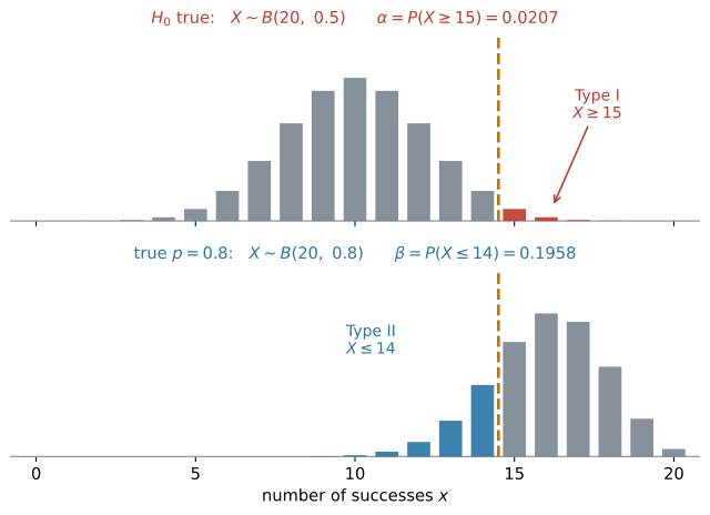
一般には、こう言います。

• Type I error … 正しい \(H_0\) を reject してしまう（rejecting \(H_0\) when \(H_0\) is true）
• Type II error … 正しくない \(H_0\) を reject しない（failing to reject \(H_0\) when \(H_0\) is false）

検定の結論（reject するかしないか）と、\(H_0\) が本当は正しいかどうかを組み合わせると、\(4\) 通りになります。

表 1: \(4\) つの場合

	\(H_0\) は本当は正しい	\(H_0\) は本当は正しくない
\(H_0\) を reject する	Type I error	正しい判断
\(H_0\) を reject しない	正しい判断	Type II error

なお、「reject しない」は「\(H_0\) が正しいと証明した」という意味ではありません（SL 4.11）。

ノート詳しく知りたい人へ（別の呼び方と、裁判のたとえ）

検査の場面では、Type I を false positive（偽陽性。何もないのに「ある」と言ってしまう）、Type II を false negative（偽陰性。あるのに「ない」と言ってしまう）と呼びます。

裁判にたとえると、\(H_0\) は「無罪」です。Type I は冤罪（無実の人を有罪にする）、Type II は取り逃がし（犯人を無罪にする）にあたります。裁判では冤罪を強く避けるので \(\alpha\) を小さく設定し、その代わり取り逃がしやすくなります。

2. The two probabilities（\(2\) つの確率を求める）

同じコインの例で、\(2\) つの確率を求めます。棄却域 \(X \geq 15\) は、どちらでも同じものを使います。

Type I error の確率。 \(H_0\) が正しい、つまり \(p = 0.5\) のときの分布で、棄却域に入る確率です。

\[ X \sim B(20,\ 0.5), \qquad P(\text{Type I}) = P(X \geq 15) = 0.0207 \]

Type II error の確率 \(\beta\)

本当は表が出やすい——たとえば本当の値が \(p = 0.8\) だとします。そのときの分布で、棄却域の外に入る確率が \(\beta\) です。

\[ X \sim B(20,\ 0.8), \qquad \beta = P(X \leq 14) = 0.196 \]

棄却域は変えません。使う分布を変えます。 上の図の \(2\) 枚は、同じ境目（\(14\) と \(15\) のあいだ）で、別々の分布を測ったものです。

表 2: \(2\) つの誤りの計算

求める確率	使う分布	求める範囲
Type I	\(H_0\) が正しいときの分布	棄却域の中
Type II	指定された本当の値での分布	棄却域の外

Type II error の確率を数値で求めるには、対立仮説に対応する具体的な母数の値が必要です。 この例の \(p = 0.8\) がそれで、問題文には if the true probability of a head is 0.8 のような形で書かれています。

指定した \(\alpha\) と、実際の確率

「significance level」ということばは、\(2\) つの意味で使われます。

• stated significance level（指定された有意水準）\(\alpha\) … 問題文が決めた値（\(5\%\) など）
• actual significance level … その棄却域で実際に \(H_0\) を棄却してしまう確率。つまり \(P(\text{Type I})\) そのもの

binomial・Poisson（離散）では、\(\alpha\) ちょうどにはなりません。 整数の境目しか選べないからです。上のコインの例でも、\(\alpha = 0.05\) と指定されているのに、実際は \(0.0207\) でした。

\[ P(\text{Type I}) \leq \alpha \quad (\text{離散分布}) \]

normal（連続）では一致します。 棄却域を丸める前の critical valueで作るので（AHL 4.18a）、面積がちょうど \(\alpha\) になります。

\[ P(\text{Type I}) = \alpha \quad (\text{連続分布}) \]

ですから Find the probability of a Type I error と問われたら、離散分布では必ず計算してください。

3. \(\beta\) is not \(1 - \alpha\)（\(\beta\) は \(1 - \alpha\) ではない）

「\(\alpha = 0.05\) なら \(\beta = 0.95\)」——これが、この項目でいちばん多い誤解です。コインの例でも \(0.0207\) と \(0.196\) で、足しても \(1\) になりません。

\(2\) つは、使っている分布が違うからです。

• \(1 - \alpha\) … \(H_0\) が正しいときに、棄却しない確率（ここでは、実際の Type I error の確率が \(\alpha\) に等しい場合を考えています）
• \(\beta\) … 指定された本当の値のもとで、\(H_0\) が誤っているときに、棄却しない確率

同じ分布の中と外なら足して \(1\) になりますが、この \(2\) つは使う分布が違います。

\(1 - \beta\) には名前があり、power（検出力）といいます。「\(H_0\) が正しくないときに、ちゃんと棄却できる確率」です。

4. Normal distribution with known variance（分散が分かっている正規分布）

\(\alpha\) と \(\beta\) を計算するのは、分散が分かっている正規分布・二項分布・ポアソン分布の \(3\) つです。\(\sigma\) が分からない \(t\) 検定では計算しません。

正規分布では、\(1\) つの値ではなく標本平均 \(\bar{X}\) の分布を使います（AHL 4.15）。その標準偏差は standard error \(\dfrac{\sigma}{\sqrt{n}}\) で、本当の値に取りかえても standard error は変わりません。動くのは中心だけです。

図 2: \(\alpha\) と \(\beta\) が表す部分です。

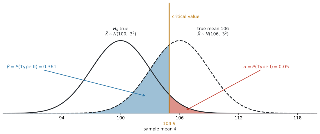
図 2 は、\(\mu_0 = 100\)、\(\sigma = 15\)、\(n = 25\)、片側 \(5\%\) の例です。実線が \(H_0\) の分布、破線が本当の平均が \(106\) のときの分布で、赤い部分が \(\alpha\)、青い部分が \(\beta\) です。別々の曲線の上で測っています。

critical value は、丸める前の値を使ってください。 \(104.9346\ldots\) を \(104.9\) に丸めて計算すると、\(\beta\) が \(0.361\) ではなく \(0.357\) になります（AHL 4.18a）。

例題 1 The mass of a bag of sugar is normally distributed with standard deviation \(\sigma = 15\) grams. The stated mean is \(100\) grams. A consumer group suspects the mean is greater than \(100\) grams and tests, at the \(5\%\) significance level, using a random sample of \(25\) bags.

(a) Find the critical value of \(\bar{x}\).

(b) Write down the probability of a Type I error.

(c) Find the probability of a Type II error if the true mean is \(106\) grams.

(d) The test is repeated at the \(1\%\) significance level. Find the new probability of a Type II error when the true mean is \(106\) grams, and comment on your answer.

日本語訳

砂糖の袋の重さは standard deviation \(\sigma = 15\) グラムの正規分布にしたがいます。表示されている平均は \(100\) グラムです。消費者団体は平均が \(100\) グラムより大きいと疑い、無作為に選んだ \(25\) 袋を使って有意水準 \(5\%\) で検定します。

(a) \(\bar{x}\) の critical value を求めなさい。

(b) Type I error の確率を書きなさい。

(c) 本当の平均が \(106\) グラムのとき、Type II error の確率を求めなさい。

(d) 有意水準 \(1\%\) で同じ検定をやり直します。本当の平均が \(106\) グラムのときの Type II error の確率を新たに求め、答えについて論評しなさい。

ヒント解説と解答例

(a) standard error は

\[ \frac{\sigma}{\sqrt{n}} = \frac{15}{\sqrt{25}} = 3 \]

片側 \(5\%\)、上側なので \(z_{\text{crit}} = 1.645\)（AHL 4.18a）。

\[ \bar{x}_{\text{crit}} = 100 + 1.645 \times 3 = 104.9346\ldots \approx 104.9 \]

(b) normal distribution（正規分布）は連続なので、critical region の面積はちょうど \(\alpha\) です。

\[ P(\text{Type I}) = 0.05 \]

計算は要りません。

(c) 手順どおりに進めます。

1. 棄却域を確認する … \(\bar{x} \geq 104.9346\ldots\)（(a) の丸める前の値）
2. 使用する分布を書く … 本当の平均が \(106\) なので \(\bar{X} \sim N(106,\ 3^2)\)。standard error は \(3\) のまま、中心だけが動きます。
3. 求める確率を書く … 棄却域の外なので \(P(\bar{X} < 104.9346\ldots)\)
4. 計算する

Normal Cdf:   Lower Bound: -∞   Upper Bound: 104.9346
              μ: 106      σ: 3

\[ \beta = P(\bar{X} < 104.9346 \mid \mu = 106) = 0.361 \]

(d) \(1\%\) なら \(z_{\text{crit}} = 2.326\) です。

\[ \bar{x}_{\text{crit}} = 100 + 2.326 \times 3 = 106.9790\ldots \approx 107.0 \]

\[ \beta = P(\bar{X} < 106.9790 \mid \mu = 106) = 0.628 \]

試験ではこう書く

Lowering the significance level from \(5\%\) to \(1\%\) moves the critical value further from \(100\), which makes the critical region smaller.

The probability of a Type I error falls from \(0.05\) to \(0.01\), but the probability of a Type II error rises from \(0.361\) to \(0.628\).

With the same sample size, reducing one type of error increases the other.

（有意水準を \(5\%\) から \(1\%\) に下げると critical value が \(100\) からさらに離れ、critical region が小さくなる。Type I error の確率は \(0.05\) から \(0.01\) に下がるが、Type II error の確率は \(0.361\) から \(0.628\) に上がる。標本の大きさが同じなら、一方の誤りを減らすともう一方が増える、という意味です。）

検算。 \(\beta\) が \(0.361\) から \(0.628\) へ増えました ✓ 表 5 と同じ向きです。

(c) と (d) で、\(\mu\) は同じ \(106\) です。 変えたのは有意水準だけなので、\(\bar{X} \sim N(106,\ 3^2)\) は同じまま、比べる境目だけが \(104.9\) から \(107.0\) に動きます。

ノート解答例（答案用紙にはこう書く）

(a) \[ \frac{\sigma}{\sqrt{n}} = \frac{15}{\sqrt{25}} = 3 \] \[ \bar{x}_{\text{crit}} = 100 + 1.645 \times 3 = 104.9346\ldots \approx 104.9 \ \text{g} \]

(b) \[ P(\text{Type I}) = 0.05 \]

(c) If \(\mu = 106\), then \(\bar{X} \sim N(106,\ 3^2)\). \[ P(\text{Type II}) = P(\bar{X} < 104.9346) = 0.361 \]

(d) \[ \bar{x}_{\text{crit}} = 100 + 2.326 \times 3 = 106.9790\ldots, \qquad P(\text{Type II}) = P(\bar{X} < 106.9790) = 0.628 \] Lowering \(\alpha\) from \(0.05\) to \(0.01\) raises \(\beta\) from \(0.361\) to \(0.628\): with the same sample size, reducing one type of error increases the other.

5. Binomial and Poisson distributions（二項分布とポアソン分布）

離散分布でも、やることは第1節のコインの例と同じです。\(H_0\) の分布で棄却域の中、本当の値の分布で棄却域の外を求めます。なお、二項分布とポアソン分布の検定は、片側検定だけが出ます。

境目の扱いに気をつけてください。 棄却域が \(X \geq 15\) なら、その外は \(X \leq 14\) です。電卓には \(0\) から \(14\) を入れます。\(X \leq 15\) とすると、\(15\) を二重に数えます（AHL 4.18b）。

例題 2 The number of accidents at a road junction follows a Poisson distribution with a mean of \(3\) per month. After a change to the traffic lights, the council tests whether the mean has increased, using the number of accidents in one month and a \(5\%\) significance level.

(a) Show that the critical region is \(X \geq 7\).

(b) Find the probability of a Type I error.

(c) Find the probability of a Type II error if the true mean is \(5\) per month.

(d) Explain what a Type II error would mean in this context.

日本語訳

ある交差点の事故の件数は、\(1\) か月あたり平均 \(3\) 件のポアソン分布にしたがいます。信号を変えたあと、自治体は平均が増えたかどうかを、\(1\) か月の事故件数と有意水準 \(5\%\) を使って検定します。

junction は「交差点」、traffic lights は「信号」、council は「自治体」という意味です。

(a) critical region が \(X \geq 7\) であることを示しなさい。

(b) Type I error の確率を求めなさい。

(c) 本当の平均が \(1\) か月あたり \(5\) 件のとき、Type II error の確率を求めなさい。

(d) この場面で Type II error が何を意味するかを説明しなさい。

ヒント解説と解答例

(a) \(H_0\): \(m = 3\)、\(H_1\): \(m > 3\)。\(H_0\) のもとで \(X \sim \mathrm{Po}(3)\) です。

表 3: Poisson の critical region

\(k\)	\(P(X \geq k)\)	\(0.05\) 以下か
\(6\)	\(0.0839\)	いいえ
\(7\)	\(\mathbf{0.0335}\)	はい

\(k = 6\) では超えてしまい、\(k = 7\) で初めて \(0.05\) 以下になります。critical region は \(X \geq 7\) です。

(b)

\[ P(\text{Type I}) = P(X \geq 7 \mid m = 3) = 0.0335 \]

(c) 手順どおりに進めます。

1. 棄却域を確認する … \(X \geq 7\)
2. 使用する分布を書く … 本当の平均が \(5\) なので \(X \sim \mathrm{Po}(5)\)
3. 求める確率を書く … 棄却域の外なので \(P(X \leq 6)\)
4. 計算する

Poisson Cdf:   λ: 5   Lower Bound: 0   Upper Bound: 6

\[ \beta = P(X \leq 6 \mid m = 5) = 0.762 \]

(d)

試験ではこう書く

A Type II error would mean that the mean number of accidents has actually increased after the change to the traffic lights, but the council fails to detect this and concludes that there is no evidence of an increase.

The dangerous junction would then be left unchanged.

（Type II error は、信号を変えたあとで事故の平均件数が実際には増えているのに、自治体がそれに気づかず、増加の証拠はないと結論してしまうことを意味する。その場合、危険な交差点はそのまま放置される、という意味です。）

\(\beta = 0.762\) は、とても大きい値です。 本当は事故が増えているのに、\(76\%\) の確率で気づけません。\(1\) か月ぶんしか見ていないので、\(\mathrm{Po}(3)\) と \(\mathrm{Po}(5)\) の見分けがつきにくいからです。\(3\) か月ぶんを見れば \(m_0 = 9\)、\(m_1 = 15\) になり、はるかに見分けやすくなります（AHL 4.17）。

ノート解答例（答案用紙にはこう書く）

(a) Under \(H_0\), \(X \sim \mathrm{Po}(3)\). \[ P(X \geq 6) = 0.0839 > 0.05, \qquad P(X \geq 7) = 0.0335 < 0.05 \] So the critical region is \(X \geq 7\).

(b) \[ P(\text{Type I}) = P(X \geq 7 \mid m = 3) = 0.0335 \]

(c) If \(m = 5\), then \(X \sim \mathrm{Po}(5)\). \[ P(\text{Type II}) = P(X \leq 6 \mid m = 5) = 0.762 \]

(d) A Type II error means the mean number of accidents has really increased but the test does not detect it, so the council wrongly concludes there is no evidence of an increase and leaves the junction unchanged.

6. Errors after a test（検定のあとに起こりえた誤り）

\(\alpha\) も \(\beta\) も、標本をとる前の確率です。結論を出したあとは、起こりえた誤りは片方だけに決まります。

表 4: 結論を出したあとに起こりえた誤り

検定の結論	起こりえた誤り
\(H_0\) を棄却した	Type I
\(H_0\) を棄却しなかった	Type II

Type I は「reject してしまう」誤りなので、reject しなかったのなら起こりようがありません。Type II は「reject しない」誤りなので、reject したのなら起こりようがありません。State which error could have occurred と問われたら、自分がどちらの結論を出したかを先に確かめてください。

なお、\(\alpha\) や \(\beta\) は、今回出した結論が間違っている確率ではありません。 同じ方法をくり返し使ったときに、どれくらいまちがえるかを表す値です。

7. The trade-off between \(\alpha\) and \(\beta\)（\(\alpha\) と \(\beta\) の関係）

標本の大きさが同じなら、\(2\) つを同時に小さくすることはできません。

図 3: \(\alpha\) を小さくすると、\(\beta\) が大きくなります。

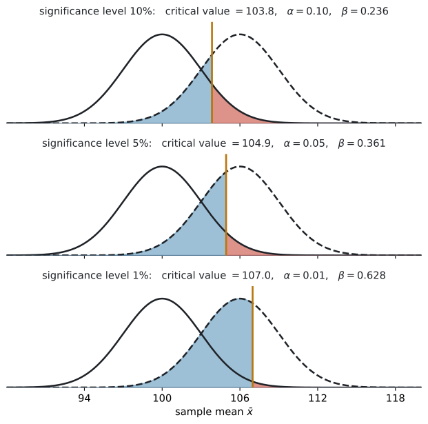
図 3 の \(3\) 枚は、同じ \(2\) 本の曲線です。動いているのは境目だけです。

表 5: \(\alpha\) を下げると \(\beta\) が上がる

significance level	critical value	\(\alpha\)	\(\beta\)
\(10\%\)	\(103.8\)	\(0.10\)	\(0.236\)
\(5\%\)	\(104.9\)	\(0.05\)	\(0.361\)
\(1\%\)	\(107.0\)	\(0.01\)	\(0.628\)

\(\alpha\) を小さくするには、境目を外へ動かします。すると赤い部分は小さくなりますが、青い部分が大きくなります。 同じ条件で棄却域を狭めると、誤って棄却しにくくなる一方で、本当の違いを見逃しやすくなるということです。

両方を小さくする代表的な方法は、標本を大きくすることです。 \(n\) が大きくなると standard error \(\dfrac{\sigma}{\sqrt{n}}\) が小さくなり、\(2\) 本の曲線が細くなります。中心は動きませんが、細くなるぶん重なりが減るので、有意水準をそのままにすれば \(\beta\) が小さくなります。

どちらの誤りが困るかは、場面で決まります。数学だけでは決められません。

表 6: どちらが重いか

場面	重い誤り	なぜ
新しい薬に副作用があるかの検査	Type II（見逃す）	危険な薬を売ってしまう
医療機器の異常を知らせる警報	Type II（見逃す）	患者が危険にさらされる
有罪かどうかの裁判	Type I（冤罪）	無実の人を罰する
工場で製品を全部作り直すかの判断	Type I	問題ないのに大きな費用がかかる

Comment on which type of error is more serious と問われたら、場面のことばで理由を書いてください。 「Type I のほうが重い」だけでは点になりません。

Why it works

ヒントクリックすると開きます

なぜ \(\beta\) には「本当の値」が要るのか

\(H_0\) は \(\mu = 100\) のように、\(1\) つの数を指定します。ですから「\(H_0\) が正しいときの分布」は \(1\) つに決まります。\(\alpha\) が計算できるのは、そのおかげです。

\(H_1\) は \(\mu > 100\) のように、範囲を指定します。\(100.1\) も \(200\) も、どちらも \(H_1\) に含まれます。

「\(H_1\) が正しいときの分布」は、\(1\) つに決まりません。 ですから \(\beta\) も \(1\) つに決まりません。

図 2 の設定では、\(\mu = 101\) なら \(\beta = 0.905\)、\(\mu = 110\) なら \(\beta = 0.0457\) です。

本当の平均が \(H_0\) から遠いほど、見逃しにくくなります。 これは感覚とも合っています。「\(1\) g の差」より「\(10\) g の差」のほうが気づきやすい、ということです。

だから問題文は、必ず特定の値を指定します。それがないと \(\beta\) という数が存在しません。

Common errors

警告\(\beta = 1 - \alpha\) としてしまう

\(2\) つは別の分布の上にあります（第3節）。足して \(1\) にはなりません。

警告\(\beta\) の計算で、\(H_0\) の値のまま電卓に入れる

\(\beta\) を出すときは、本当の値に入れ替えます（第3節）。

第1節 のコインの例なら、Prob Success を \(0.5\) から \(0.8\) に変えます。

警告離散分布で \(P(\text{Type I}) = 0.05\) と書く

離散では \(\alpha\) ちょうどになりません（第2節）。計算してください。

第1節 のコインの例では \(0.0207\)、例 2 では \(0.0335\) です。

警告critical region の外の範囲を、\(1\) つずらす

\(X \geq 15\) の外は \(X \leq 14\) です。\(X \leq 15\) ではありません（第5節）。

警告\(\beta\) の計算で standard error を変えてしまう

正規分布では、本当の平均に変えても \(\dfrac{\sigma}{\sqrt{n}}\) はそのままです（第4節）。動くのは中心だけです。

警告\(\alpha\) を下げれば \(\beta\) も下がると考える

逆です。\(\alpha\) を下げると \(\beta\) は上がります（第7節）。

警告Type I と Type II を取り違える

Type I は「正しい \(H_0\) を reject」、Type II は「間違った \(H_0\) を reject しない」です。

動いてしまったほうが Type I（reject する）、動かなかったほうが Type II（reject しない）。reject のうしろに「しない」が付くかどうかで見分けてください（表 1）。

警告どちらが重いかを、場面のことばで書かない

Type I is more serious だけでは点になりません。「その場面で何が起きるか」を書いてください（第7節）。

警告検定のあとで、両方の誤りが起こりえたと書く

\(H_0\) を棄却したなら Type I、棄却しなかったなら Type II——起こりえるのは片方だけです（第6節）。

警告\(\beta\) を求めるのに、本当の値を問題文から探さない

\(\beta\) は本当の値がないと計算できません（第3節）。Find the probability of a Type II error とあれば、問題文に具体的な値が与えられているはずです。 それが無いと、\(\beta\) は数値では求まりません。

警告\(t\) 検定で Type II error を計算しようとする

Type II error の確率を計算するのは、正規分布（分散が分かっているとき）・ポアソン分布・二項分布だけです（第4節）。\(t\) 検定では計算しません。

Using your GDC (TI-Nspire CX II)

新しいコマンドはありません。 AHL 4.18a と AHL 4.18b で使ったものを、分布の数字だけ入れ替えてもう一度使います。

Discrete distributions（離散分布のとき）

\(2\) 回、Cdf を使います。

第1節 のコインの例なら、critical region は \(X \geq 15\) です。

① Type I:    Binomial Cdf   n: 20   p: 0.5   Lower: 15   Upper: 20
② Type II:   Binomial Cdf   n: 20   p: 0.8   Lower: 0    Upper: 14

変わるのは \(2\) か所です。p と、範囲の向き。

表 7: 離散での入力

	p	Lower	Upper
Type I	\(H_0\) の値	critical region の下端	上限
Type II	本当の値	\(0\)	critical region の下端 \(-1\)

ヒントUpper を \(1\) 引くところがポイントです

critical region が \(X \geq 15\) なら、その外は \(X \leq 14\)。Upper Bound は \(14\) です。

\(15\) と入れると、critical region の \(1\) 本ぶんを二重に数えます。

Normal distributions（正規分布のとき）

Normal Cdf を使います（SL 4.9）。

Normal Cdf:   Lower Bound: -∞      Upper Bound: 104.9346
              μ: 106      σ: 3

表 8: 正規分布での入力

欄	入れるもの
μ	本当の平均（\(H_0\) の値ではない）
σ	standard error \(\dfrac{\sigma}{\sqrt{n}}\)
範囲	critical region の外

警告σ の欄に \(\sigma\) をそのまま入れないでください

\(\bar{X}\) の散らばりは \(\dfrac{\sigma}{\sqrt{n}}\) です。例 1 なら \(3\) であって、\(15\) ではありません。

\(15\) を入れると \(\beta = 0.472\) となり、答えが変わってしまいます。

ヒント\(-\infty\) の出し方

Lower Bound に端がないときは、\(-\infty\) を入れます。\(\infty\) は、キーボードのいちばん下、左端の π のキーを押すと開く記号パレットから選びます（AHL 1.12a と同じパレットです）。\(-\infty\) は、負号 (-) を打ってから \(\infty\) を選びます。

\(-1E99\) と入れても同じです（\(-1 \times 10^{99}\) という意味で、EE キーで出します。SL 4.9）。

Inverse Normal と違い、Normal Cdf は両側の境目を要求するので、片側だけのときもここを埋めます。

Exercises

1 A test of \(H_0: p = 0.4\) against \(H_1: p > 0.4\) uses a sample of size \(25\) and the critical region \(X \geq 15\).

(a) Find the probability of a Type I error.

(b) Find the probability of a Type II error if the true value of \(p\) is \(0.6\).

日本語訳

\(H_0: p = 0.4\) を \(H_1: p > 0.4\) に対して検定します。標本の大きさは \(25\) で、critical region は \(X \geq 15\) です。

(a) Type I error の確率を求めなさい。

(b) \(p\) の本当の値が \(0.6\) のとき、Type II error の確率を求めなさい。

ノート解答例（答案用紙に書くこと）

(a) Under \(H_0\), \(X \sim B(25,\ 0.4)\). \[ P(\text{Type I}) = P(X \geq 15 \mid p = 0.4) = 0.0344 \]

(b) If \(p = 0.6\), then \(X \sim B(25,\ 0.6)\). \[ P(\text{Type II}) = P(X \leq 14 \mid p = 0.6) = 0.414 \]

ヒント解説

(a) \(H_0\) の値 \(p = 0.4\) で計算します（第2節）。

Binomial Cdf:   n: 25   p: 0.4   Lower: 15   Upper: 25

(b) 本当の値 \(p = 0.6\) に入れ替えます（第3節）。範囲は critical region の外、つまり \(X \leq 14\) です。

Binomial Cdf:   n: 25   p: 0.6   Lower: 0   Upper: 14

検算。 \(0.0344\) と \(0.414\) を足しても \(1\) になりません ✓ なってはいけません（第3節）。

この critical region は AHL 4.18a の例題3 と同じものです。

2 A test of \(H_0: m = 6\) against \(H_1: m > 6\) for a Poisson distribution uses the critical region \(X \geq 11\).

(a) Find the probability of a Type I error.

(b) Find the probability of a Type II error if the true mean is \(10\).

日本語訳

ポアソン分布について \(H_0: m = 6\) を \(H_1: m > 6\) に対して検定します。critical region は \(X \geq 11\) です。

(a) Type I error の確率を求めなさい。

(b) 本当の平均が \(10\) のとき、Type II error の確率を求めなさい。

ノート解答例（答案用紙に書くこと）

(a) Under \(H_0\), \(X \sim \mathrm{Po}(6)\). \[ P(\text{Type I}) = P(X \geq 11 \mid m = 6) = 0.0426 \]

(b) If \(m = 10\), then \(X \sim \mathrm{Po}(10)\). \[ P(\text{Type II}) = P(X \leq 10 \mid m = 10) = 0.583 \]

ヒント解説

(a) \(\mathrm{Po}(6)\) で \(X \geq 11\)。Upper Bound は \(100\) など大きい数にします（AHL 4.18a）。

(b) \(\mathrm{Po}(10)\) に入れ替え、\(X \leq 10\) の確率です。

Poisson Cdf:   λ: 10   Lower: 0   Upper: 10

警告(b) の \(10\) が \(2\) か所に出ますが、意味が違います

λ: 10 の \(10\) は本当の平均、Upper: 10 の \(10\) は critical region の下端 \(11\) から \(1\) 引いた数です。

偶然、同じ数になっています。混ざらないように、\(1\) つずつ確かめてください。

検算。 \(\beta = 0.583\) は大きめです。\(\mathrm{Po}(6)\) と \(\mathrm{Po}(10)\) はまだ形が近いので、\(1\) 回の観測では見分けにくい——それが数に出ています ✓

3 The time taken to process an application is normally distributed with standard deviation \(\sigma = 6\) minutes. The office claims a mean of \(50\) minutes. A manager tests, at the \(5\%\) significance level, whether the mean is greater than \(50\) minutes, using a random sample of \(36\) applications.

(a) Find the critical value of \(\bar{x}\).

(b) Write down the probability of a Type I error.

(c) Find the probability of a Type II error if the true mean is \(52\) minutes.

日本語訳

ある申請の処理にかかる時間は standard deviation \(\sigma = 6\) 分の正規分布にしたがいます。この事務所は平均 \(50\) 分だと主張しています。ある管理者が、無作為に選んだ \(36\) 件の申請を使い、平均が \(50\) 分より大きいかどうかを有意水準 \(5\%\) で検定します。

application は「申請」という意味です。

(a) \(\bar{x}\) の critical value を求めなさい。

(b) Type I error の確率を書きなさい。

(c) 本当の平均が \(52\) 分のとき、Type II error の確率を求めなさい。

ノート解答例（答案用紙に書くこと）

(a) \[ \frac{\sigma}{\sqrt{n}} = \frac{6}{\sqrt{36}} = 1 \] \[ \bar{x}_{\text{crit}} = 50 + 1.645 \times 1 = 51.6449\ldots \approx 51.6 \ \text{minutes} \]

(b) \[ P(\text{Type I}) = 0.05 \]

(c) If \(\mu = 52\), then \(\bar{X} \sim N(52,\ 1^2)\). \[ P(\text{Type II}) = P(\bar{X} < 51.6449) = 0.361 \]

ヒント解説

(a) standard error は \(\dfrac{6}{6} = 1\) です。

\[ 50 + 1.645 \times 1 = 51.6449 \ldots \]

\(3\) 桁で \(51.6\) です。

(b) 正規分布は連続なので、ちょうど \(0.05\) です（第2節）。計算しません。

(c) 中心を \(52\) に動かします。standard error は \(1\) のままです（第4節）。

Normal Cdf:   Lower: -∞   Upper: 51.6449   μ: 52   σ: 1

\[ \beta = 0.361 \]

ヒント\(\beta\) が 例 1 と同じ \(0.361\) になりました

偶然ではありません。どちらも片側 \(5\%\) で、例 1 は「\(\mu_0\) から \(6\)、standard error が \(3\)」、この問題は「\(\mu_0\) から \(2\)、standard error が \(1\)」——どちらも standard error \(2\) 個ぶん離れています。

同じ有意水準なら、\(\beta\) を決めるのは「本当の値が \(\mu_0\) から standard error 何個ぶん離れているか」だけです。実際の単位や \(n\) ではありません。

有意水準が変われば、同じ距離でも \(\beta\) は変わります（第7節）。

検算。 丸めた \(51.6\) ではなく \(51.6449\) で計算しました。丸めた \(51.6\) を使うと \(0.345\) になり、\(2\) 桁目からずれます ✓ \(\beta\) の計算では、丸める前の critical value を使ってください。

4 A factory tests batches of components. \(H_0\) is that a batch meets the required standard.

For each of the following, state whether it describes a Type I error, a Type II error, or a correct decision.

(a) A batch that meets the standard is rejected.

(b) A batch that does not meet the standard is accepted for sale.

(c) A batch that does not meet the standard is rejected.

(d) For one particular batch the test does not reject \(H_0\). State which type of error could have occurred, and which could not.

日本語訳

ある工場が部品のまとまりを検査しています。\(H_0\) は「そのまとまりが required standard を満たしている」です。

batch は「まとまり、ロット」、component は「部品」、meet the standard は「基準を満たす」という意味です。

次のそれぞれが、Type I error か Type II error か、それとも正しい判断かを述べなさい。

(a) 基準を満たしているまとまりが、不合格にされる。

(b) 基準を満たしていないまとまりが、販売用に受け入れられる。

(c) 基準を満たしていないまとまりが、不合格にされる。

(d) ある \(1\) つのまとまりについて、検定は \(H_0\) を棄却しませんでした。どちらの種類の誤りが起こりえたか、またどちらが起こりえないかを述べなさい。

ノート解答例（答案用紙に書くこと）

(a) A Type I error: \(H_0\) is true but is rejected.

(b) A Type II error: \(H_0\) is false but is not rejected.

(c) A correct decision: \(H_0\) is false and is rejected.

(d)

A Type II error could have occurred, because \(H_0\) was not rejected and a Type II error is failing to reject a false \(H_0\).

A Type I error could not have occurred, because that requires \(H_0\) to be rejected.

（Type II error が起こりえた。\(H_0\) が棄却されておらず、Type II error は誤った \(H_0\) を棄却しないことだからである。Type I error は起こりえない。それには \(H_0\) が棄却されている必要があるからである、という意味です。）

ヒント解説

\(H_0\) が何かを、はっきりさせるのが先です。 ここでは「基準を満たしている」が \(H_0\) です。

表 1 に当てはめます。

(a) 基準を満たしている（\(H_0\) は正しい）のに不合格（reject）→ Type I

(b) 満たしていない（\(H_0\) は正しくない）のに受け入れた（reject しない）→ Type II

(c) 満たしていない（\(H_0\) は正しくない）ので不合格（reject）→ 正しい判断

(d) 結論を出したあとの問いです（第6節）。

\(H_0\) を棄却しなかったのだから、「棄却してしまう」誤り（Type I）は起こりようがありません。

残るのは Type II だけです。表 4 を見てください。

「起こりえた」であって、「起きた」ではありません。 聞かれているのは、起こりえたのはどちらか、です。

警告「不合格」が reject に対応します

日常の「合格・不合格」と、検定の「reject する・しない」は向きが逆に感じられます。

このまとまりを不合格にするということは、「基準を満たしている」という \(H_0\) を否定したということです。

毎回、\(H_0\) が何かに戻って考えてください。

5 A student writes:

“The test is carried out at the \(5\%\) significance level, so the probability of a Type I error is \(0.05\) and the probability of a Type II error is \(0.95\).”

Explain the error in this reasoning.

日本語訳

ある生徒がこう書きました。

「有意水準 \(5\%\) で検定するので、Type I error の確率は \(0.05\)、Type II error の確率は \(0.95\) である。」

この理由づけの誤りを説明しなさい。

ノート解答例（答案用紙に書くこと）

The two probabilities are calculated under different distributions, so they do not add to \(1\).

\(P(\text{Type I})\) is found assuming \(H_0\) is true, while \(P(\text{Type II})\) is found assuming a specific alternative value is true.

A Type II error cannot even occur when \(H_0\) is true.

In addition, \(P(\text{Type II})\) cannot be found at all until a particular alternative value is given, so it is not determined by the significance level.

（\(2\) つの確率は別々の分布のもとで計算されるので、足して \(1\) にはならない。\(P(\text{Type I})\) は \(H_0\) が正しいという仮定のもとで求め、\(P(\text{Type II})\) は特定の対立仮説の値が正しいという仮定のもとで求める。\(H_0\) が正しいときには Type II error は起こりえない。さらに、\(P(\text{Type II})\) は特定の対立仮説の値が与えられるまで求めることすらできないので、有意水準では決まらない、という意味です。）

ヒント解説

誤りは \(2\) つあります。両方書いてください。

\(1\) つめ。\(\beta = 1 - \alpha\) ではありません（第3節）。\(2\) つは別の分布の上にあるので、足す意味がありません。

\(2\) つめ。そもそも \(\beta\) は、有意水準だけでは決まりません。 本当の値が与えられないと計算できません（第3節）。

\(1\) つめだけ書くと、半分の答えになります。「\(0.95\) が違う」だけでなく、「そもそも数が決まらない」まで書いてください。

なお \(P(\text{Type I}) = 0.05\) のほうは、正規分布なら正しいです。離散分布なら、これも違います（第2節）。

6 A quantity is normally distributed with standard deviation \(\sigma = 10\). A test of \(H_0: \mu = 200\) against \(H_1: \mu > 200\) uses a random sample of \(25\).

(a) Find the critical value of \(\bar{x}\) at the \(5\%\) significance level, and the probability of a Type II error when the true mean is \(205\).

(b) Find the critical value of \(\bar{x}\) and the probability of a Type II error at the \(1\%\) significance level.

(c) Comment on your answers.

日本語訳

ある量は standard deviation \(\sigma = 10\) の正規分布にしたがいます。\(H_0: \mu = 200\) を \(H_1: \mu > 200\) に対して、無作為に選んだ \(25\) 個の標本で検定します。

(a) 有意水準 \(5\%\) での \(\bar{x}\) の critical value と、本当の平均が \(205\) のときの Type II error の確率を求めなさい。

(b) 有意水準 \(1\%\) での \(\bar{x}\) の critical value と Type II error の確率を求めなさい。

(c) 答えについて論評しなさい。

ノート解答例（答案用紙に書くこと）

\[ \frac{\sigma}{\sqrt{n}} = \frac{10}{\sqrt{25}} = 2 \]

(a) \[ \bar{x}_{\text{crit}} = 200 + 1.645 \times 2 = 203.2897\ldots \approx 203.3 \] \[ P(\text{Type II}) = P(\bar{X} < 203.2897 \mid \mu = 205) = 0.196 \]

(b) \[ \bar{x}_{\text{crit}} = 200 + 2.326 \times 2 = 204.6527\ldots \approx 204.7 \] \[ P(\text{Type II}) = P(\bar{X} < 204.6527 \mid \mu = 205) = 0.431 \]

(c)

Lowering the significance level from \(5\%\) to \(1\%\) reduces the probability of a Type I error from \(0.05\) to \(0.01\), but it raises the probability of a Type II error from \(0.196\) to \(0.431\).

With a fixed sample size the two cannot both be made small, so the choice of significance level depends on which error matters more in the situation.

（有意水準を \(5\%\) から \(1\%\) に下げると Type I error の確率は \(0.05\) から \(0.01\) に減るが、Type II error の確率は \(0.196\) から \(0.431\) に上がる。標本の大きさが決まっていれば \(2\) つを同時に小さくはできないので、有意水準の選び方は、その場面でどちらの誤りが重いかによる、という意味です。）

ヒント解説

standard error は \(\dfrac{10}{5} = 2\) で、(a) (b) 共通です。

(a) \(200 + 1.645 \times 2 = 203.2897\ldots\)

Normal Cdf:   Lower: -∞   Upper: 203.2897   μ: 205   σ: 2

\[ \beta = 0.196 \]

(b) \(200 + 2.326 \times 2 = 204.6527\ldots\)

\[ \beta = 0.431 \]

(c) \(\beta\) が \(0.196\) から \(0.431\) へ、\(2\) 倍以上に増えました。

この対比が、この問題の中心です（第7節）。「どちらの誤りを避けたいか」で有意水準を選ぶ、というところまで書いてください。

検算。 \(\alpha\) を下げたら \(\beta\) が上がりました ✓ 逆になっていたら、どこかで分布か範囲を取り違えています。

7 A test of \(H_0: m = 4\) against \(H_1: m > 4\) for a Poisson distribution uses the critical region \(X \geq 9\).

(a) Find the probability of a Type II error when the true mean is (i) \(6\), (ii) \(8\), (iii) \(10\).

(b) Describe how the probability of a Type II error changes as the true mean increases, and explain why.

日本語訳

ポアソン分布について \(H_0: m = 4\) を \(H_1: m > 4\) に対して検定します。critical region は \(X \geq 9\) です。

(a) 本当の平均が (i) \(6\)、(ii) \(8\)、(iii) \(10\) のときの Type II error の確率を求めなさい。

(b) 本当の平均が増えるにつれて Type II error の確率がどう変わるかを述べ、その理由を説明しなさい。

ノート解答例（答案用紙に書くこと）

(a) The critical region is \(X \geq 9\), so a Type II error occurs when \(X \leq 8\).

(i) \(P(X \leq 8 \mid m = 6) = 0.847\)

(ii) \(P(X \leq 8 \mid m = 8) = 0.593\)

(iii) \(P(X \leq 8 \mid m = 10) = 0.333\)

(b)

The probability of a Type II error decreases as the true mean increases.

When the true mean is far from the value in \(H_0\), the observed count is much more likely to fall in the critical region, so the test is much more likely to detect that \(H_0\) is false.

A small departure from \(H_0\) is hard to detect; a large one is easy.

（本当の平均が大きくなるにつれて Type II error の確率は減る。本当の平均が \(H_0\) の値から遠いと、観測される件数が critical region に入る可能性がずっと高くなるので、検定が \(H_0\) の誤りを見つけられる可能性がずっと高くなる。\(H_0\) からのわずかなずれは見つけにくく、大きなずれは見つけやすい、という意味です。）

ヒント解説

(a) critical region が \(X \geq 9\) なので、その外は \(X \leq 8\) です。\(\lambda\) だけを \(6\)、\(8\)、\(10\) と入れ替えます。

Poisson Cdf:   λ: 6    Lower: 0   Upper: 8      →  0.847
Poisson Cdf:   λ: 8    Lower: 0   Upper: 8      →  0.593
Poisson Cdf:   λ: 10   Lower: 0   Upper: 8      →  0.333

Upper: 8 は \(3\) 回とも同じです。critical region は変わっていません。

(b) \(0.847 \to 0.593 \to 0.333\) と減っています。

理由は Why it works で見たことです。\(H_0\) から遠いほど、見逃しにくい。

検算。 単調に減っています ✓ 増えていたら、\(\lambda\) と Upper を取り違えています。

8 A test of \(H_0: p = 0.25\) against \(H_1: p > 0.25\) uses a sample of size \(30\) at the \(5\%\) significance level.

(a) Show that the critical region is \(X \geq 13\).

(b) Find the probability of a Type I error, and explain why it is not \(0.05\).

(c) Find the probability of a Type II error if the true value of \(p\) is \(0.5\).

日本語訳

\(H_0: p = 0.25\) を \(H_1: p > 0.25\) に対して、大きさ \(30\) の標本を使い有意水準 \(5\%\) で検定します。

(a) critical region が \(X \geq 13\) であることを示しなさい。

(b) Type I error の確率を求め、それが \(0.05\) でない理由を説明しなさい。

(c) \(p\) の本当の値が \(0.5\) のとき、Type II error の確率を求めなさい。

ノート解答例（答案用紙に書くこと）

(a) Under \(H_0\), \(X \sim B(30,\ 0.25)\). \[ P(X \geq 12) = 0.0507 > 0.05, \qquad P(X \geq 13) = 0.0216 < 0.05 \] So the critical region is \(X \geq 13\).

(b) \[ P(\text{Type I}) = P(X \geq 13 \mid p = 0.25) = 0.0216 \]

\(X\) can only take whole-number values, so the probability of the critical region changes in jumps and cannot be made exactly \(0.05\).

The region is chosen to be the largest whose probability is still less than \(0.05\), and here that probability is \(0.0216\).

（\(X\) は整数の値しか取れないので critical region の確率は飛び飛びに変わり、ちょうど \(0.05\) にはできない。region は確率が \(0.05\) を超えない範囲でいちばん大きいものが選ばれ、ここではその確率が \(0.0216\) である、という意味です。）

(c) If \(p = 0.5\), then \(X \sim B(30,\ 0.5)\). \[ P(\text{Type II}) = P(X \leq 12 \mid p = 0.5) = 0.181 \]

ヒント解説

(a) \(P(X \geq 12) = 0.0507\) で、\(0.05\) をわずかに超えます。 ですから \(X \geq 13\) です（AHL 4.18a）。

この設定は AHL 4.18a の演習4 と、AHL 4.18b の演習8 と同じです。\(3\) ページで同じ場面を、違う角度から見ています。

(b) \(0.0216\) です。\(0.05\) の半分以下になっています。

これは「損をしている」ようにも見えますが、\(0.05\) を超える region は使えないのでやむを得ません（第2節）。

(c) \(p = 0.5\) に入れ替え、\(X \leq 12\) です。

Binomial Cdf:   n: 30   p: 0.5   Lower: 0   Upper: 12

\[ \beta = 0.181 \]

検算。 \(H_0\) のもとでの平均は \(30 \times 0.25 = 7.5\)、本当の値では \(30 \times 0.5 = 15\) です。\(15\) は critical region（\(X \geq 13\)）の中にあるので、\(\beta\) が小さめ（\(0.181\)）になるのは正しい向きです ✓

9 A hospital screening test is used to decide whether a patient should be referred for further investigation. Let \(H_0\) be that the patient does not have the condition.

(a) Describe, in context, what a Type I error and a Type II error would mean.

(b) Comment on which type of error is more serious in this situation.

日本語訳

ある病院の検診が、患者をさらに詳しい検査に回すべきかどうかを決めるのに使われています。\(H_0\) は「その患者はその病気ではない」とします。

screening test は「検診」、refer for further investigation は「さらに詳しい検査に回す」、condition はここでは「病気」という意味です。

(a) Type I error と Type II error が、この場面で何を意味するかを述べなさい。

(b) この場面ではどちらの誤りがより重大かを論評しなさい。

ノート解答例（答案用紙に書くこと）

(a)

A Type I error means that a patient who does not have the condition is referred for further investigation.

A Type II error means that a patient who does have the condition is not referred, so the condition is missed.

（Type I error は、その病気ではない患者がさらに詳しい検査に回されることを意味する。Type II error は、その病気である患者が回されず、病気が見逃されることを意味する、という意味です。）

(b)

A Type II error is more serious here, because a patient who has the condition would go untreated and their health could deteriorate.

A Type I error causes unnecessary further testing, which costs money and causes the patient anxiety, but it is usually corrected at the next stage.

For this reason a screening test is often set up with a fairly large significance level, accepting more Type I errors in order to make Type II errors rare.

（ここでは Type II error のほうが重大である。病気である患者が治療されないままになり、健康が悪化しうるからだ。Type I error は不要な追加検査を招き、費用がかかり患者に不安を与えるが、ふつうは次の段階で訂正される。このため検診は、Type II error をまれにするために Type I error が増えるのを受け入れて、やや大きめの有意水準で設定されることが多い、という意味です。）

ヒント解説

この問題に計算はありません。 Describe, in context と Comment on は、どちらもことばで答える問いです。

(a) の型は決まっています。

• Type I …「\(H_0\) が正しいのに reject」を、場面のことばに直す
• Type II …「\(H_0\) が正しくないのに reject しない」を、場面のことばに直す

「\(H_0\) を棄却する」と書いてはいけません。 「検査に回す」「回さない」という、この場面のことばに直してください。

(b) には、決まった正解はありません。 ただし理由が要ります。

「Type II のほうが重い」と書くだけでは点になりません。「病気が見逃されて治療されない」という結果まで書いて、はじめて理由になります。

ヒント両方の誤りの結果を並べると、強い答えになります

片方だけ書くより、「Type I ならこうなる、Type II ならこうなる、だからこちらが重い」と並べたほうが説得力があります。

上の解答例は、その形になっています。

10 A bag of coffee beans should have a mean mass of \(25\) grams. The mass is normally distributed with standard deviation \(\sigma = 2\) grams. A supervisor tests, at the \(5\%\) significance level, whether the machine is underfilling, using a random sample of \(16\) bags.

(a) Find the critical region for \(\bar{x}\).

(b) Write down the probability of a Type I error.

(c) Find the probability of a Type II error if the true mean is \(23.5\) grams.

(d) State one change the supervisor could make that would reduce both types of error, and explain why it works.

日本語訳

コーヒー豆の袋は平均 \(25\) グラムであるべきです。重さは standard deviation \(\sigma = 2\) グラムの正規分布にしたがいます。ある管理者が、無作為に選んだ \(16\) 袋を使って、機械が少なく詰めているかどうかを有意水準 \(5\%\) で検定します。

coffee beans は「コーヒー豆」、underfill は「規定より少なく詰める」という意味です。

(a) \(\bar{x}\) の critical region を求めなさい。

(b) Type I error の確率を書きなさい。

(c) 本当の平均が \(23.5\) グラムのとき、Type II error の確率を求めなさい。

(d) \(2\) 種類の誤りを両方とも減らすために管理者ができる変更を \(1\) つ述べ、それが効く理由を説明しなさい。

ノート解答例（答案用紙に書くこと）

(a) \[ H_0: \mu = 25, \qquad H_1: \mu < 25 \] \[ \frac{\sigma}{\sqrt{n}} = \frac{2}{\sqrt{16}} = 0.5 \] \[ \bar{x}_{\text{crit}} = 25 - 1.645 \times 0.5 = 24.1776\ldots \approx 24.2 \] Critical region: \(\bar{x} < 24.2\) g.

(b) \[ P(\text{Type I}) = 0.05 \]

(c) If \(\mu = 23.5\), then \(\bar{X} \sim N(23.5,\ 0.5^2)\). \[ P(\text{Type II}) = P(\bar{X} > 24.1776) = 0.0877 \]

(d)

The supervisor could take a larger sample.

Increasing \(n\) reduces the standard error \(\sigma / \sqrt{n}\), so both distributions become narrower and overlap less.

At the same significance level the probability of a Type II error becomes much smaller, and because of that the supervisor could also lower the significance level, so that both error probabilities end up smaller than before.

（管理者は標本を大きくすればよい。\(n\) を増やすと standard error \(\sigma / \sqrt{n}\) が小さくなるので、\(2\) つの分布はどちらも細くなり、重なりが減る。同じ有意水準のままなら Type II error の確率が大きく下がり、そのぶん有意水準も下げられるので、結果として \(2\) 種類の誤りの確率を両方とも前より小さくできる、という意味です。）

ヒント解説

(a) 「少なく詰めている」なので下側です。\(z_{\text{crit}} = -1.645\)（AHL 4.18a）。

standard error は \(\dfrac{2}{4} = 0.5\)。

\[ 25 - 1.645 \times 0.5 = 24.1776\ldots \]

\(3\) 桁で \(24.2\) です。

(b) 連続なので、ちょうど \(0.05\) です。

(c) 下側の検定なので、critical region の外は「上」です。\(\bar{x} > 24.177\ldots\) の確率を出します。

Normal Cdf:   Lower: 24.1776   Upper: ∞   μ: 23.5   σ: 0.5

\[ \beta = 0.0877 \]

警告上側の問題と、範囲の向きが逆になります

これまでの例題は上側の検定だったので、\(\beta\) は「境目より下」でした。

この問題は下側の検定なので、\(\beta\) は「境目より上」です。

critical region の外がどちらかを、毎回、絵を描いて確かめてください。

(d) 第7節の最後に書いた、標本を大きくする話のことです。

有意水準を動かすだけでは、片方しか減らせません。 両方減らすには、分布そのものを細くするしかありません。

\(n\) を大きくすれば、\(\dfrac{\sigma}{\sqrt{n}}\) が小さくなります。

\(\sigma\) は population（母集団）の性質なので、勝手に変えられません。変えられるのは \(n\) だけです。

検算。 \(\beta = 0.0877\) は小さめです。本当の平均 \(23.5\) は critical value \(24.2\) より下にあり、つまり critical region の中にあります。見つけやすい状況なので、\(\beta\) が小さいのは正しい向きです ✓